PyTorch Beginner’s Guide: Autograd, Gradient Descent, detach(), and Linear Regression Training - Devuly | Smart Analytics for Developers & Projects

This article focuses on practical PyTorch fundamentals. It explains autograd, gradient descent, tensor detachment with detach(), and the full linear regression training workflow, helping beginners move beyond writing code to truly understanding backpropagation and parameter updates. Keywords: PyTorch, autograd, linear regression.

Table of Contents

The technical specification snapshot summarizes the stack and task scope.

Parameter	Description
Language	Python
Core Framework	PyTorch
Task Type	Automatic differentiation, optimization, regression modeling
Typical Protocols / Paradigms	Backpropagation, SGD, MSELoss
Star Count	Not provided in the source
Core Dependencies	`torch`, `torch.nn`, `torch.optim`, `matplotlib`, `scikit-learn`

PyTorch’s core training mechanism can be broken down into autograd and parameter updates.

PyTorch has a relatively low learning curve largely because of its dynamic computation graph and automatic differentiation system. Developers only need to declare requires_grad=True, and the framework records the computation path automatically, then computes gradients during backward().

During training, a model does not directly “learn the answer.” Instead, it measures prediction error through a loss function and continuously adjusts parameters based on gradients. In essence, this process is numerical optimization.

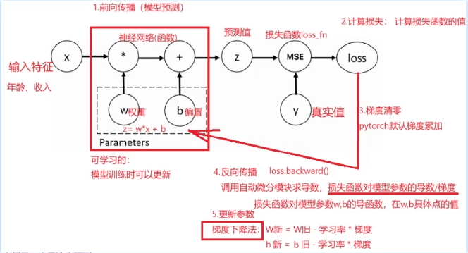AI Visual Insight: This image shows where automatic differentiation sits inside the training loop: input features and weights participate in the forward pass, the loss function measures error, backpropagation produces gradients, and the learning rate updates parameters, forming an iterative training cycle.

The standard autograd workflow should be understood as a fixed template.

Define trainable parameters such as weight w and bias b.
Run the forward pass to obtain predictions.
Compute the loss.
Clear old gradients to prevent gradient accumulation from contaminating the current iteration.
Call backward() to run backpropagation.
Read grad and update parameters.

import torch

# 1. Set a fixed random seed for reproducibility
torch.manual_seed(5)

# 2. Build inputs and targets
x = torch.ones(2, 5)
y = torch.zeros(2, 1)

# 3. Define trainable parameters and enable autograd
w = torch.rand(5, 1, requires_grad=True)
b = torch.rand(1, requires_grad=True)

# 4. Forward pass: linear computation z = xw + b
z = x @ w + b

# 5. Define the loss function and compute loss
loss_fn = torch.nn.MSELoss()
loss = loss_fn(z, y)

# 6. Zero gradients: PyTorch accumulates gradients by default
if w.grad is not None:
    w.grad.zero_()  # Clear old weight gradients
if b.grad is not None:
    b.grad.zero_()  # Clear old bias gradients

# 7. Backpropagation: compute gradients automatically
loss.backward()

# 8. Manually update parameters
w.data -= 0.01 * w.grad.data  # Update weights using the learning rate
b.data -= 0.01 * b.grad.data  # Update bias using the learning rate

This code demonstrates the smallest complete PyTorch training loop, from graph construction and differentiation to parameter updates.

Gradient descent fundamentally moves parameters in the direction opposite to the steepest increase in loss.

When a loss function is differentiable with respect to its parameters, the gradient gives the direction of steepest ascent at the current position. To reduce the loss, you update parameters in the opposite direction of the gradient. That is why the common formula is: W_new = W_old - lr * grad.

The original example uses loss = w**2 + 20 to demonstrate how to search for a minimum. Because the derivative is 2w, the loss reaches its minimum when w approaches 0. This is an excellent example for understanding optimizer behavior.

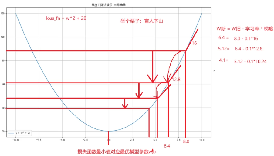AI Visual Insight: This figure represents how the loss function changes with the parameter value, emphasizing that gradient descent does not jump directly to the optimum. Instead, it uses local derivative information to gradually approach the minimum region, illustrating how the learning rate and number of iterations affect convergence speed.

Minimal code can clearly show how parameters approach the optimum step by step.

import torch

# Define initial parameters and enable gradients
w = torch.tensor([10.0, 20.0], requires_grad=True, dtype=torch.float32)
loss_list = []

for i in range(500):
    # Forward pass: define the objective function
    loss = w ** 2 + 20

    # Zero gradients to avoid accumulation
    if w.grad is not None:
        w.grad.zero_()

    # Backpropagate the mean loss
    loss.mean().backward()

    # Update parameters by moving against the gradient
    w.data = w.data - 0.01 * w.grad

    # Save the loss for later plotting
    loss_list.append(loss.mean().item())

This example shows that even without a complex neural network, PyTorch can directly solve numerical optimization problems.

The core value of detach is that it breaks the computation graph so you can safely convert tensors to NumPy.

Many beginners try to call .numpy() directly on a tensor with requires_grad=True, which raises an error. The root cause is not a type mismatch. The tensor is still attached to the computation graph, and PyTorch does not allow it to be exposed directly to NumPy.

The correct approach is to call detach() first. It returns a new tensor that no longer participates in gradient propagation, and you can then safely convert it to a NumPy array.

import torch

# Create a tensor that tracks gradients
w = torch.tensor([1.0, 2.0, 3.0], requires_grad=True, dtype=torch.float32)

# Break the computation graph first, then convert to numpy
n2 = w.detach().numpy()

# Modify the numpy array and observe whether memory is shared
n2[0] = 28.0
print(w)
print(n2)

This example verifies that detach().numpy() often returns a shallow-copy view, so modifying the NumPy array may affect the original tensor contents.

During inference and visualization, `detach` is a high-frequency operation.

For example, when you pass model outputs to matplotlib for plotting or to scikit-learn for additional analysis, you typically need to call detach() first. Otherwise, conversion fails because the tensor still depends on the gradient graph.

When building linear regression with PyTorch, the recommended pattern combines Dataset, DataLoader, nn.Module, and an optimizer.

Although linear regression is simple, it already covers the standard infrastructure of deep learning training: dataset packaging, batch loading, model definition, loss computation, backpropagation, optimizer updates, and training visualization.

This practice uses make_regression-style synthetic one-dimensional regression data and fits the underlying line with nn.Linear(1,1). This pattern transfers naturally to more complex training tasks such as MLPs, CNNs, and Transformers.

import torch
from torch.utils.data import TensorDataset, DataLoader
from torch import nn, optim

# Build the dataset
x = torch.randn(100, 1)
y = 3.5 * x + 13.9 + torch.randn(100, 1)

# Wrap the data loader
loader = DataLoader(TensorDataset(x, y), batch_size=16, shuffle=True)

# Define the linear model, loss function, and optimizer
model = nn.Linear(1, 1)
loss_fn = nn.MSELoss()
optimizer = optim.SGD(model.parameters(), lr=0.01)

for epoch in range(100):
    for x_train, y_train in loader:
        # Forward pass
        y_pred = model(x_train)
        loss = loss_fn(y_pred, y_train)

        # Zero gradients
        optimizer.zero_grad()

        # Backpropagation
        loss.backward()

        # Update model parameters
        optimizer.step()

This code shows the minimal standard pattern for framework-based PyTorch training and works well as a template for supervised learning tasks.

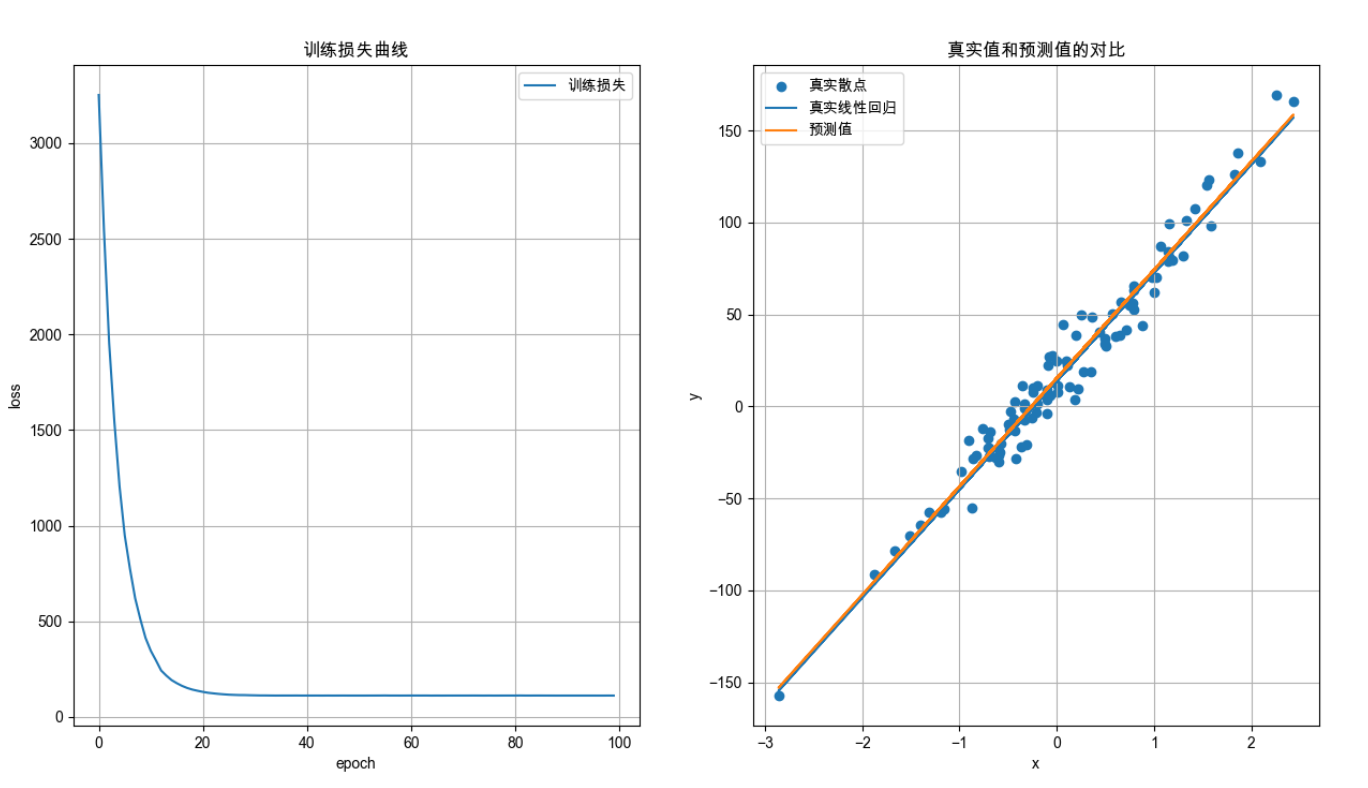AI Visual Insight: This figure compares the true sample scatter plot, the theoretical regression line, and the model prediction curve after training. You can use it to judge whether the model has correctly fitted the one-dimensional linear relationship and whether the loss reduction translates into interpretable prediction accuracy.

The key observations in the training workflow determine how quickly you can debug issues.

First, check whether the loss decreases steadily. If it does not, inspect the learning rate, label dimensions, and gradient reset logic first. Next, check whether predictions follow the same overall trend as the real data distribution. If even the direction is wrong, the problem usually lies in data preprocessing or input dimensions.

Also, understanding the order of optimizer.zero_grad(), loss.backward(), and optimizer.step() is critical. If the order is wrong, parameters may fail to update or gradients may accumulate incorrectly.

FAQ

1. Why do I need to zero gradients before every backward pass in PyTorch?

Because PyTorch accumulates gradients by default. If you do not clear them, gradients from the previous iteration will be added to the current gradients, leading to incorrect parameter updates.

2. Why can’t a tensor with `requires_grad=True` be converted directly to NumPy?

Because that tensor is still connected to the automatic differentiation graph. Converting it directly to NumPy would break the graph structure, so you must use detach() first to remove the gradient dependency.

3. What is the most common source of errors in linear regression training?

The most common issues are mismatched label dimensions, forgetting zero_grad(), using an unreasonable learning rate, and mixing training-stage tensor logic with inference-stage conversion logic.

Core Summary: This article systematically reconstructs the core concepts of practical PyTorch usage, covering autograd, gradient descent, detach, and the linear regression training workflow to help developers build a complete mental model from tensor differentiation to model optimization.