Object Detection Data Augmentation Explained: Practical Strategies from Geometric Transforms to Mosaic, CutMix, and ISDA

[AI Readability Summary] For object detection and vision training workloads, data augmentation helps address limited samples, heavy occlusion, hard-to-detect small objects, and long-tail class distributions. This article organizes augmentation techniques into pixel-level, occlusion-level, cross-sample mixing, and feature-level methods, and provides implementation-ready code. Keywords: object detection, data augmentation, Mosaic

The technical specification snapshot outlines the scope

Parameter	Description
Topic	Image data augmentation in object detection
Primary language	Python
Core libraries	OpenCV, NumPy, PyTorch
Applicable tasks	Detection, segmentation, classification, industrial vision
Common frameworks	YOLO family, general CV training pipelines
License/source	Compiled from blog content; no open-source license declared
Star count	Not provided
Core dependencies	cv2, numpy, torch, torch.nn

Data augmentation is the lowest-cost way to raise the ceiling of object detection

In vision model training, data quality directly determines generalization. Compared with simply adding more model parameters, data augmentation is a better fit for projects with limited samples, constrained compute, and highly variable scenes.

Its essence is not to “create more images,” but to expose the model to a richer distribution: viewpoint changes, lighting variation, partial occlusion, background perturbation, and semantic composition across images.

Geometric and pixel-level augmentation form the basic layer of robustness

Geometric augmentation mainly addresses viewpoint and scale variation, while pixel-level augmentation mainly addresses sensor and environmental variation. In practice, both are default components in most training pipelines.

import cv2
import numpy as np

def aug_geometric(img: np.ndarray) -> dict:
    h, w = img.shape[:2]
    results = {}
    results["HorizontalFlip"] = cv2.flip(img, 1)  # Horizontal flip to simulate left-right viewpoint changes
    results["VerticalFlip"] = cv2.flip(img, 0)    # Vertical flip for specific top-down scenarios

    M = cv2.getRotationMatrix2D((w // 2, h // 2), 45, 1.0)
    results["Rotate45"] = cv2.warpAffine(img, M, (w, h))  # Rotate by 45 degrees

    cy, cx = int(h * 0.15), int(w * 0.15)
    crop = img[cy:h - cy, cx:w - cx]
    results["CenterCrop70%"] = cv2.resize(crop, (w, h))   # Center crop and resize back to the original size
    return results

This code shows how flipping, rotation, and crop-resize expand the spatial distribution of targets.

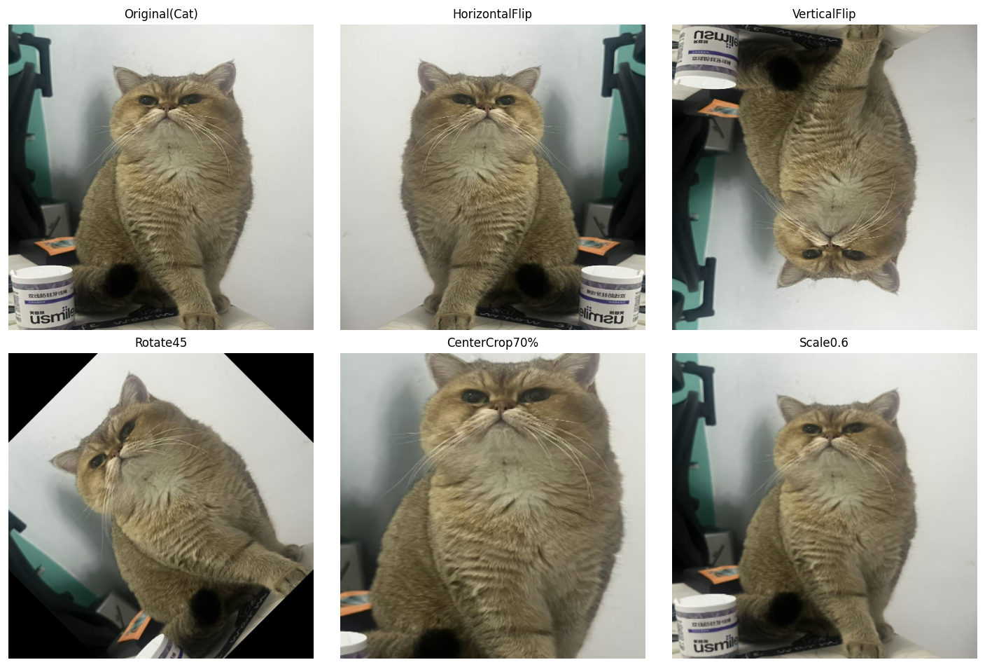
AI Visual Insight: This figure shows the visual differences produced by multiple geometric augmentations on the same target, including flipping, rotation, cropping, and scaling. It makes one point clear: augmentation does not change the semantic class, but it does significantly change bounding box positions, object scale, and local context. In object detection training, you must transform annotation coordinates in sync with the image.

def aug_color_jitter(img: np.ndarray) -> dict:
    results = {}
    hsv = cv2.cvtColor(img, cv2.COLOR_RGB2HSV).astype(np.float32)

    bright = np.clip(img.astype(np.float32) + 60, 0, 255).astype(np.uint8)
    results["Brightness+60"] = bright  # Increase brightness to simulate strong lighting

    contrast = np.clip(img.astype(np.float32) * 1.8, 0, 255).astype(np.uint8)
    results["Contrastx1.8"] = contrast  # Increase contrast to enhance edge differences

    hsv[..., 1] = np.clip(hsv[..., 1] * 2, 0, 255)
    results["Saturationx2"] = cv2.cvtColor(hsv.astype(np.uint8), cv2.COLOR_HSV2RGB)
    return results

This code simulates changes in brightness, contrast, and saturation to improve model adaptability under different imaging conditions.

Occlusion-focused augmentation reduces model reliance on local texture

When targets in a dataset are frequently occluded, the model can overfit to local texture cues. The value of Random Erasing and GridMask is that they force the model to learn global structure instead of local shortcuts.

def aug_random_erasing(img: np.ndarray, erase_ratio: float = 0.15, fill: int = 128) -> np.ndarray:
    out = img.copy()
    h, w = out.shape[:2]
    eh, ew = int(h * erase_ratio), int(w * erase_ratio)
    top = np.random.randint(0, h - eh)
    left = np.random.randint(0, w - ew)
    out[top:top + eh, left:left + ew] = fill  # Randomly erase a local region
    return out

This code improves recognition of incomplete targets by randomly occluding local regions.

GridMask and CutMix both strengthen discrimination under occlusion

GridMask is well suited to segmentation and dense prediction tasks because its occlusion pattern is regular. CutMix is often a better fit for detection because it changes both local pixels and label proportions.

def aug_cutmix(img_a: np.ndarray, img_b: np.ndarray, cut_ratio: float = 0.3) -> np.ndarray:
    out = img_a.copy()
    h, w = out.shape[:2]
    ch, cw = int(h * cut_ratio), int(w * cut_ratio)
    top = np.random.randint(0, h - ch)
    left = np.random.randint(0, w - cw)
    out[top:top + ch, left:left + cw] = img_b[top:top + ch, left:left + cw]  # Replace a local region
    return out

This code pastes a local patch from another image into the current sample to improve robustness to occlusion and boundary discrimination.

Cross-sample mixing is one of the most effective gain drivers in the YOLO family

Mixup, CutMix, and Mosaic share one common trait: they turn single-image training into multi-image joint supervision. This can significantly improve background diversity, target density, and small-object recall.

def aug_mixup(img_a: np.ndarray, img_b: np.ndarray, alpha: float = 0.4) -> np.ndarray:
    lam = np.random.beta(alpha, alpha)
    mixed = lam * img_a.astype(np.float32) + (1 - lam) * img_b.astype(np.float32)  # Linearly blend two images
    return np.clip(mixed, 0, 255).astype(np.uint8)

def aug_mosaic(imgs: list) -> np.ndarray:
    assert len(imgs) >= 4, "Mosaic requires at least 4 images"
    h, w = imgs[0].shape[:2]
    top = np.concatenate([imgs[0], imgs[1]], axis=1)
    bottom = np.concatenate([imgs[2], imgs[3]], axis=1)
    mosaic = np.concatenate([top, bottom], axis=0)  # Stitch four images into a dense sample
    return cv2.resize(mosaic, (w, h))

This code demonstrates transparent blending and four-image stitching. Both approaches expand the training distribution and improve robustness in complex backgrounds.

Long-tail classes and small datasets benefit more from Copy-Paste and ISDA

When some classes have very few samples, the gains from standard flipping and cropping are limited. Copy-Paste directly increases the appearance frequency of rare targets, while ISDA creates “reasonable perturbations” in feature space.

import torch
import torch.nn as nn

class ISDALoss(nn.Module):
    def __init__(self, feature_num, class_num):
        super().__init__()
        self.estimator = EstimatorCV(feature_num, class_num)  # Maintain class-level feature statistics

    def forward(self, features, y, target_layer):
        self.estimator.update_CV(features, y)  # Update mean and covariance estimates
        logits = target_layer(features)
        isda_logits = logits + self.estimator.get_purturb(features, y)  # Apply perturbation in feature space
        return nn.CrossEntropyLoss()(isda_logits, y)

This code shows that ISDA does not directly modify pixels. Instead, it improves generalization in feature space during loss computation.

Augmentation strategy selection should map directly to the business pain point

If your task focuses on small objects and long-range detection, prioritize Mosaic + Mixup. If the main issue is occlusion and complex backgrounds, prioritize CutMix + GridMask. If you face long-tail classes and sample scarcity, Copy-Paste + ISDA usually provides better cost-effectiveness.

Business pain point	Recommended strategy
Small objects, long-range detection	Mosaic + Mixup
Object occlusion, noisy backgrounds	CutMix + GridMask
Very few samples, long-tail classes	Copy-Paste + ISDA

Production pipelines must update annotations and control distribution shift

In object detection, augmentation does not apply only to images. Any operation involving cropping, stitching, rotation, or patch pasting must also update bounding boxes, masks, or keypoints. Otherwise, you will corrupt the training data.

At the same time, stronger augmentation is not always better. Excessive color perturbation, overly aggressive erasing, or excessively dense Mosaic composition can shift the training distribution away from the real deployment environment and ultimately hurt online performance.

FAQ

Q1: Which augmentations are most worth enabling first in object detection?

A1: If you do not have strong scene constraints, start with random flipping, color jitter, Mosaic, and Mixup. This set is easy to implement, delivers stable gains, and works well as a baseline configuration.

Q2: Why can performance drop after adding data augmentation?

A2: The most common reasons are that augmentation breaks the real data distribution or annotations are not updated in sync. In detection tasks especially, incorrect bounding box transforms directly introduce noisy labels.

Q3: What is the core difference between ISDA and standard image augmentation?

A3: Standard augmentation operates in pixel space, while ISDA operates in feature space. The former changes the input image; the latter implicitly expands the semantic distribution during training through class covariance modeling.

Core Summary: This article systematically reconstructs the mainstream image augmentation methods used in object detection, covering geometric transforms, color jitter, noise injection, Random Erasing, GridMask, Mixup, CutMix, Mosaic, Copy-Paste, and ISDA, along with their use cases, core code, and strategy-combination recommendations.