This article breaks down a FreeRTOS closed-loop control pipeline for a differential drive chassis: it first converts linear and angular velocity commands through inverse kinematics, then uses dual-wheel PID controllers to track the target wheel speeds, and finally drives the motors through PWM and direction pins. It solves the practical gap between “high-level motion commands” and “actual motor actuation.” Keywords: FreeRTOS, PID closed loop, PWM motor driving.
Technical Specifications at a Glance
| Parameter | Description |
|---|---|
| Runtime Environment | STM32 + FreeRTOS |
| Implementation Language | C |
| Chassis Model | Two-wheel differential drive |
| Control Period | 10 ms |
| Velocity Inputs | vx_mmps, wz_mradps |
| Outputs | Left and right wheel PWM and direction control |
| Core Dependencies | HAL / timer PWM, GPIO, math library lroundf |
| Protocols / Interfaces | Task notifications, driver interface, wheel speed feedback interface |
| Star Count | Not provided in the source |
This control pipeline maps abstract motion commands to actual motor actuation
In a FreeRTOS control task, robot motion does not come from a single algorithm. It comes from a continuous data path: the upper layer issues velocity commands, and the lower layer completes inverse kinematics, speed regulation, and drive output. This design separates the workflow into three independent modules: “compute the target,” “track the target,” and “execute the target,” which makes the system easier to maintain and replace.
For a differential drive chassis, the upper layer usually cares only about the robot’s forward velocity and yaw rate. It does not directly specify left and right wheel speeds. The control task converts that higher-level motion intent into PWM control values that the motors can actually execute.
Inverse kinematics distributes chassis velocity to the left and right wheels
A differential drive model has no lateral velocity degree of freedom. Its inputs are typically only linear velocity vx_mmps and angular velocity wz_mradps. The controller first converts wz_mradps to rad/s, then combines it with half of the wheelbase to compute the target linear speed for each wheel.
static void diff_inverse_kinematics_mmps_mradps(int16_t vx_mmps,
                                                int16_t wz_mradps,
                                                float* vL,
                                                float* vR)
{
    float wz_rad = (float)wz_mradps / 1000.0f;      // Convert angular velocity units
    float half_base = WHEEL_BASE_MM * 0.5f;         // Compute half the wheelbase

    float vL_val = (float)vx_mmps - wz_rad * half_base; // Target speed for the left wheel
    float vR_val = (float)vx_mmps + wz_rad * half_base; // Target speed for the right wheel

    vL_val = clampf(vL_val, -MAX_WHEEL_SPEED_MMPS, MAX_WHEEL_SPEED_MMPS); // Speed limiting protection
    vR_val = clampf(vR_val, -MAX_WHEEL_SPEED_MMPS, MAX_WHEEL_SPEED_MMPS); // Speed limiting protection

    *vL = vL_val;
    *vR = vR_val;
}
This code maps robot-level velocity commands to left and right wheel target speeds, while applying safety limits before the values enter the control loop.
Its physical meaning is straightforward: during straight motion, both wheels run at the same speed; during a turn, the outer wheel runs faster and the inner wheel runs slower. The benefit of this design is that if you later change the wheelbase or chassis dimensions, you only need to update the kinematic parameters instead of rewriting the PID or driver layer.
PID closed-loop control converts target wheel speed into stable output
The result of inverse kinematics is only the speed that the wheels should reach. In reality, the motor response is affected by load, friction, and power supply variation, so it cannot follow the target precisely on its own. That is why a speed closed loop is necessary: it continuously drives the measured value toward the reference.
Each wheel maintains its own independent PID controller. The proportional term provides a fast response to the current error, the integral term removes steady-state error, and the derivative term suppresses oscillation caused by rapid changes. In the original implementation, you can set the derivative term to zero during early tuning to simplify debugging.
The PID update logic must handle both integral limiting and output limiting
static void PID_Init(PID_t* pid, float kp, float ki, float kd,
                     float i_limit, float out_limit)
{
    pid->kp = kp;
    pid->ki = ki;
    pid->kd = kd;
    pid->i_acc = 0.0f;          // Clear the initial integral value
    pid->prev_err = 0.0f;       // Clear the previous error
    pid->i_limit = i_limit;
    pid->out_limit = out_limit;
}

static int16_t PID_Update(PID_t* pid, float ref, float meas, float dt)
{
    float err = ref - meas;                         // Current speed error
    float p_out = pid->kp * err;                   // Proportional output

    pid->i_acc += pid->ki * err * dt;              // Accumulate the integral of the error
    pid->i_acc = clampf(pid->i_acc, -pid->i_limit, pid->i_limit); // Prevent integral windup

    float d_out = 0.0f;
    if (pid->kd != 0.0f && dt > 0.0f) {
        d_out = pid->kd * (err - pid->prev_err) / dt; // Compute the derivative term
    }
    pid->prev_err = err;

    float out = p_out + pid->i_acc + d_out;        // Combine the control output
    out = clampf(out, -pid->out_limit, pid->out_limit); // Limit the total output

    return clampi16((int16_t)lroundf(out), PWM_MIN, PWM_MAX); // Convert to a PWM value
}
This code generates a protected PWM control value from the difference between the target wheel speed and the measured wheel speed, preventing integral runaway and output overshoot.
The most important engineering detail here is not the formula itself, but the limiting strategy. Without i_limit, the integral term keeps accumulating under persistent error. As the system gets close to the target, the controller may still output too much control effort, which leads to obvious overshoot and oscillation.
The PWM driver layer converts logical control values into hardware behavior
The output of the PID controller is still only a logical value. To actually drive the motor, the system must coordinate the direction pins and timer PWM. Typical two-line H-bridge drivers, such as TB6612 and L298, use a “direction + duty cycle” control scheme.
In this implementation, Motor_ApplyPwm(pwmL, pwmR) is the execution entry point. It accepts logical PWM values in the range -1000~1000. The sign determines the direction, and the absolute value determines the duty cycle. This lets the upper layer focus only on control values instead of low-level GPIO states.
static void motor_apply_dir_2pin(int16_t pwm, GPIO_TypeDef* in1_port, uint16_t in1_pin,
                                 GPIO_TypeDef* in2_port, uint16_t in2_pin)
{
    if (pwm > 0) {
        HAL_GPIO_WritePin(in1_port, in1_pin, GPIO_PIN_SET);   // Forward direction
        HAL_GPIO_WritePin(in2_port, in2_pin, GPIO_PIN_RESET);
    } else if (pwm < 0) {
        HAL_GPIO_WritePin(in1_port, in1_pin, GPIO_PIN_RESET); // Reverse direction
        HAL_GPIO_WritePin(in2_port, in2_pin, GPIO_PIN_SET);
    } else {
        HAL_GPIO_WritePin(in1_port, in1_pin, GPIO_PIN_RESET); // Stop with brake/coast behavior
        HAL_GPIO_WritePin(in2_port, in2_pin, GPIO_PIN_RESET);
    }
}
This code switches the motor direction pins based on the sign of the PWM value, implementing forward rotation, reverse rotation, and stop control.
The full control flow should run at a stable fixed period
In each 10 ms control cycle, the task usually runs in a fixed sequence: read the velocity command, execute inverse kinematics, obtain wheel speed feedback, update the dual PID controllers, and apply PWM. This sequence forms a stable speed closed loop.
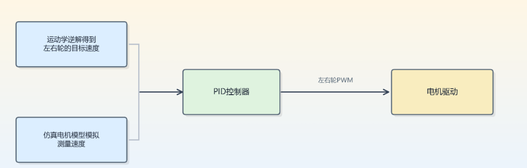 AI Visual Insight: This diagram shows the serial control chain of a differential drive chassis, from upper-layer velocity commands to actuator output. The target velocity first goes through left/right wheel distribution, then combines with wheel speed feedback and enters a dual-channel PID controller, which finally outputs left and right PWM signals to the motor driver. The diagram highlights the standard discrete closed-loop structure built from the reference value, feedback value, and control output, which maps naturally to a periodic FreeRTOS control task.
A typical periodic task framework looks like this
void ControlTask_10ms(void)
{
    float refL, refR, measL, measR;

    diff_inverse_kinematics_mmps_mradps(cmd_vx, cmd_wz, &refL, &refR); // Compute the target wheel speeds
    Motor_GetWheelSpeedMmps(&measL, &measR);                           // Read the actual wheel speeds

    int16_t pwmL = PID_Update(&pid_left, refL, measL, 0.01f);         // Closed-loop control for the left wheel
    int16_t pwmR = PID_Update(&pid_right, refR, measR, 0.01f);        // Closed-loop control for the right wheel

    Motor_ApplyPwm(pwmL, pwmR);                                       // Send the output to the driver layer
}
This code connects inverse kinematics, feedback acquisition, PID computation, and PWM output into a deterministic 10 ms control cycle.
This modular design improves system scalability
The greatest value of this solution is not only that it makes a two-wheel robot move, but that it establishes clear software boundaries. The inverse kinematics layer handles only mathematical mapping, the PID layer handles only error convergence, and the driver layer handles only hardware execution. The three layers remain loosely coupled.
That means if you later replace simulated wheel speed feedback with encoder feedback, or move from a two-wheel differential drive to another chassis structure, you can constrain the required changes to the corresponding module without breaking the overall FreeRTOS control task framework.
FAQ
Q1: Why can’t the upper layer send motor PWM directly instead of performing inverse kinematics first?
Because the upper layer describes the robot’s overall motion goal, such as forward velocity and yaw rate, while the motor actuators require wheel-level targets such as left and right wheel speed or PWM. Inverse kinematics converts a robot-level goal into wheel-level targets, which is a necessary bridge in chassis control.
Q2: Why is integral limiting required in a PID controller?
The integral term accumulates historical error. If the motor cannot reach the target for an extended period, the integral term keeps growing and causes integral windup. Even after the error decreases, the controller may still output excessive control effort, leading to overshoot, oscillation, and poor stability. That is why limiting is an engineering necessity.
Q3: Can simulated wheel speed feedback directly replace a real encoder?
No, not for long-term use. Simulated feedback works well during early integration and debugging because it helps verify closed-loop logic, interfaces, and parameter trends. In a real deployment, however, you still need encoder or Hall sensor feedback. Otherwise, the system cannot reflect real friction, load disturbances, or mechanical offsets, and control accuracy remains limited.
AI Readability Summary
This article reconstructs the execution pipeline of a differential drive chassis inside a FreeRTOS control task. It focuses on inverse kinematics, dual-wheel PID closed-loop regulation, and PWM driver interface design. It explains how target velocity becomes executable motor control output and provides a modular implementation approach suitable for STM32 and embedded systems.