UAV 3D Path Planning Algorithm Comparison: I-GWO vs GWO, GJO, SCSO, and SCA in Complex Mountain Terrain - Devuly | Smart Analytics for Developers & Projects

This article examines UAV 3D path planning in complex mountain environments and compares five intelligent optimization algorithms: GWO, I-GWO, GJO, SCSO, and SCA. The core challenges are multi-constraint obstacle avoidance, premature convergence, and insufficient trajectory smoothness. Keywords: UAV path planning, Grey Wolf Optimization, Matlab.

Table of Contents

Technical Specifications Snapshot

Parameter	Details
Research Target	UAV 3D trajectory path planning
Core Algorithms	GWO, I-GWO, GJO, SCSO, SCA
Implementation Language	Matlab
Environment Model	Digital Elevation Model + cylindrical threat zones
Trajectory Representation	Spherical coordinate parameterization
Optimization Objectives	Path length, threat avoidance, altitude control, trajectory smoothness
Experimental Method	30 independent repeated simulations
Star Count	Not provided in the original content
License	CC 4.0 BY-SA
Core Dependencies	Matlab numerical computing and 3D visualization capabilities

This study targets the path planning bottlenecks of flight in complex mountain terrain

The original study addresses the UAV 3D path planning problem in complex mountain environments. This problem is jointly constrained by terrain variation, no-fly threats, flight attitude limits, and path smoothness requirements, making it a typical high-dimensional, nonlinear, multi-constraint optimization task.

Compared with traditional geometric methods or graph search methods, swarm intelligence algorithms are better suited for such non-differentiable problems with complex constraints. The focus here is not the implementation of a single algorithm, but a unified comparative evaluation centered on the improved Grey Wolf Optimizer, I-GWO, against GWO, GJO, SCSO, and SCA under the same modeling framework.

The research problem can be abstracted into a unified cost minimization model

The path planning objective is defined as minimizing a composite cost. The cost consists of four parts: path length, threat penalty, altitude penalty, and smoothness penalty. This design balances flight efficiency, safety, and engineering feasibility.

function cost = path_cost(path, threat, terrain, weight)
    L = calc_length(path);                 % Compute total trajectory length
    T = calc_threat_penalty(path, threat); % Compute threat zone penalty
    H = calc_height_penalty(path, terrain);% Compute altitude safety penalty
    S = calc_smooth_penalty(path);         % Compute turning and climb smoothness penalty
    cost = weight(1)*L + weight(2)*T + weight(3)*H + weight(4)*S;
end

This code illustrates the core idea of the paper: map multi-objective path quality into a single composite fitness value that can be optimized directly.

Spherical coordinate representation reduces search redundancy and strengthens angular constraints

Instead of searching all trajectory points directly in 3D Cartesian coordinates, the study represents nodes in spherical coordinates. The value of this design is that each path segment is decomposed into distance, azimuth, and pitch angle, which better matches the physical characteristics of continuous UAV maneuvers.

Spherical parameterization also reduces unnecessary degrees of freedom, making it easier to enforce climb angle and turn angle constraints. For complex mountain path planning, this is a key design choice that improves convergence efficiency and trajectory feasibility, not just a simple coordinate substitution.

Constraint modeling determines whether the results have engineering value

The environment model includes three categories of constraints: terrain boundary constraints, cylindrical threat avoidance constraints, and flight dynamics constraints. In particular, the threat zones are modeled as cylinders. This simplification fits Matlab simulation well and also enables fair comparison across algorithms under identical conditions.

function flag = is_feasible(point, bound, threat)
    in_bound = point(1)>=bound.xmin && point(1)<=bound.xmax; % Check X boundary
    in_bound = in_bound && point(2)>=bound.ymin && point(2)<=bound.ymax; % Check Y boundary
    in_bound = in_bound && point(3)>=bound.zmin && point(3)<=bound.zmax; % Check Z boundary

    safe = true;
    for k = 1:length(threat)
        d = norm(point(1:2) - threat(k).center); % Compute planar distance
        if d <= threat(k).radius && point(3) <= threat(k).height
            safe = false; % Mark infeasible if the point enters a cylindrical threat zone
            break;
        end
    end
    flag = in_bound && safe;
end

This code summarizes the basic logic for feasible-solution filtering: each path node must satisfy both spatial boundary constraints and obstacle avoidance constraints.

The improvements in I-GWO come from three coordinated mechanisms rather than a single patch

The standard GWO suffers from a linearly decreasing convergence factor, limited local exploitation accuracy in later iterations, and difficulty escaping local optima once the population clusters. To address this, the paper designs I-GWO as a three-layer improvement structure rather than replacing only one parameter.

The first improvement is a nonlinear convergence factor. It preserves stronger global exploration in the early stage and then contracts more quickly toward high-quality local regions in the later stage. The second is adaptive perturbation, which helps relieve stagnation. The third is Cauchy mutation, which uses a heavy-tailed distribution to strengthen the ability to escape local extrema.

Nonlinear convergence and mutation strategies jointly shape convergence quality

The key to this type of improvement is not formula complexity, but search rhythm control. Through a “diffuse first, focus later, then perturb” mechanism, I-GWO is more likely to discover short, smooth, and safe paths in a complex cost landscape.

for t = 1:maxIter
    a = 2 * sin(pi/2 * (1 - t/maxIter));   % Nonlinear convergence factor
    for i = 1:popSize
        Xnew = gwo_update(X(i,:), Alpha, Beta, Delta, a); % Grey Wolf position update
        step = randn(size(Xnew)) * (1 - t/maxIter);       % Adaptive perturbation step size
        Xnew = Xnew + step;                               % Perturbation-enhanced local search
        Xnew = cauchy_mutation(Xnew);                     % Cauchy mutation to escape local optima
        X(i,:) = bound_fix(Xnew, lb, ub);                 % Boundary correction to ensure feasibility
    end
end

This process snippet captures the key I-GWO execution loop: update, perturb, mutate, and correct.

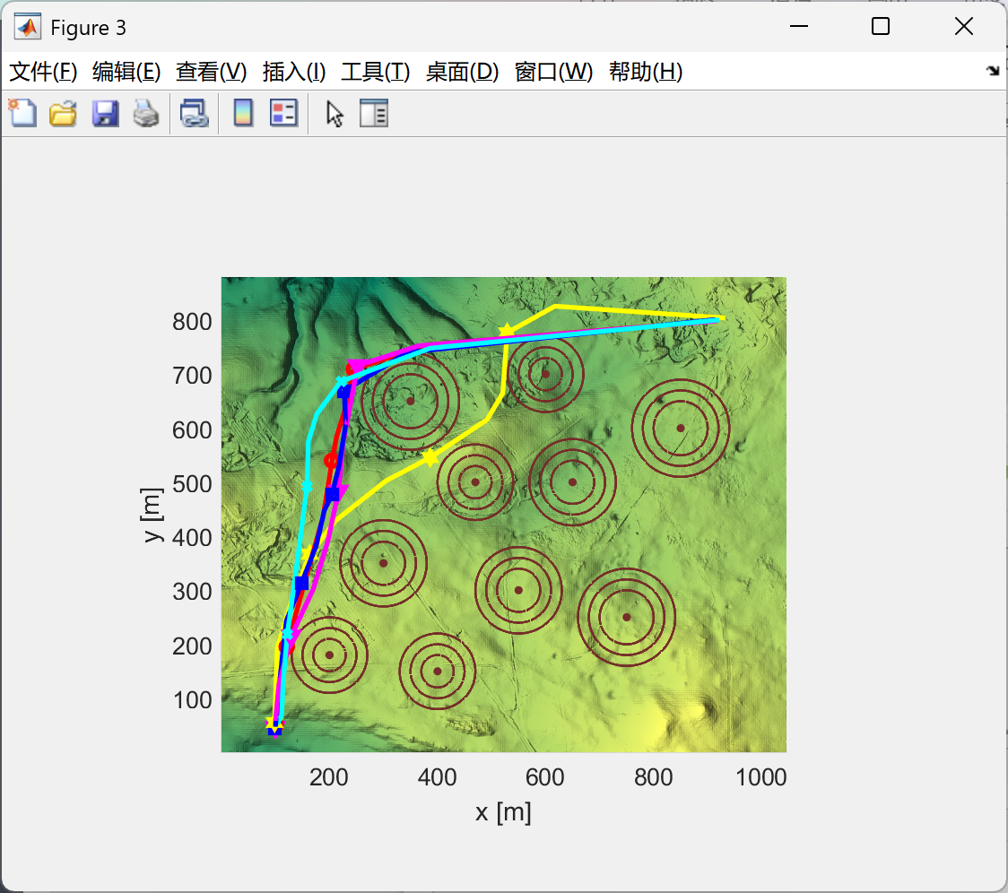
Comparative experiments show that I-GWO performs better in both accuracy and stability

The conclusions reported in the original content are very clear: across 30 independent repeated experiments, I-GWO outperformed GWO, GJO, SCSO, and SCA on four statistical metrics: best value, mean value, standard deviation, and worst value. This indicates not only better best-case solutions, but also stronger stability.

These results matter more for engineering deployment. A path planning algorithm should not be judged only by a single best run; it must also demonstrate consistency across repeated runs. A smaller standard deviation means the algorithm does not depend heavily on a lucky initialization and is therefore more suitable for batch execution in real systems.

The Matlab output snippet reflects the statistical evaluation method

The original article provides a short result-printing snippet, showing that the experiments use a unified statistical framework to compare five algorithms. Although simple, this style is highly effective for reproducing the study’s conclusions.

disp(['iGWO Best: ', num2str(iGWObest)]);    % Output I-GWO best value
disp(['iGWO Mean: ', num2str(iGWOmean)]);    % Output I-GWO mean value
disp(['iGWO Std: ', num2str(iGWOstd)]);      % Output I-GWO standard deviation
disp(['GWO Best: ', num2str(GWObest)]);      % Output GWO best value
disp(['GJO Best: ', num2str(GJObest)]);      % Output GJO best value
disp(['SCSO Best: ', num2str(SCSObest)]);    % Output SCSO best value
disp(['SCA Best: ', num2str(SCAbest)]);      % Output SCA best value

The purpose of this code is to output unified multi-algorithm statistics for horizontal comparison of optimality and robustness.

Three-dimensional result plots further validate the differences in path quality

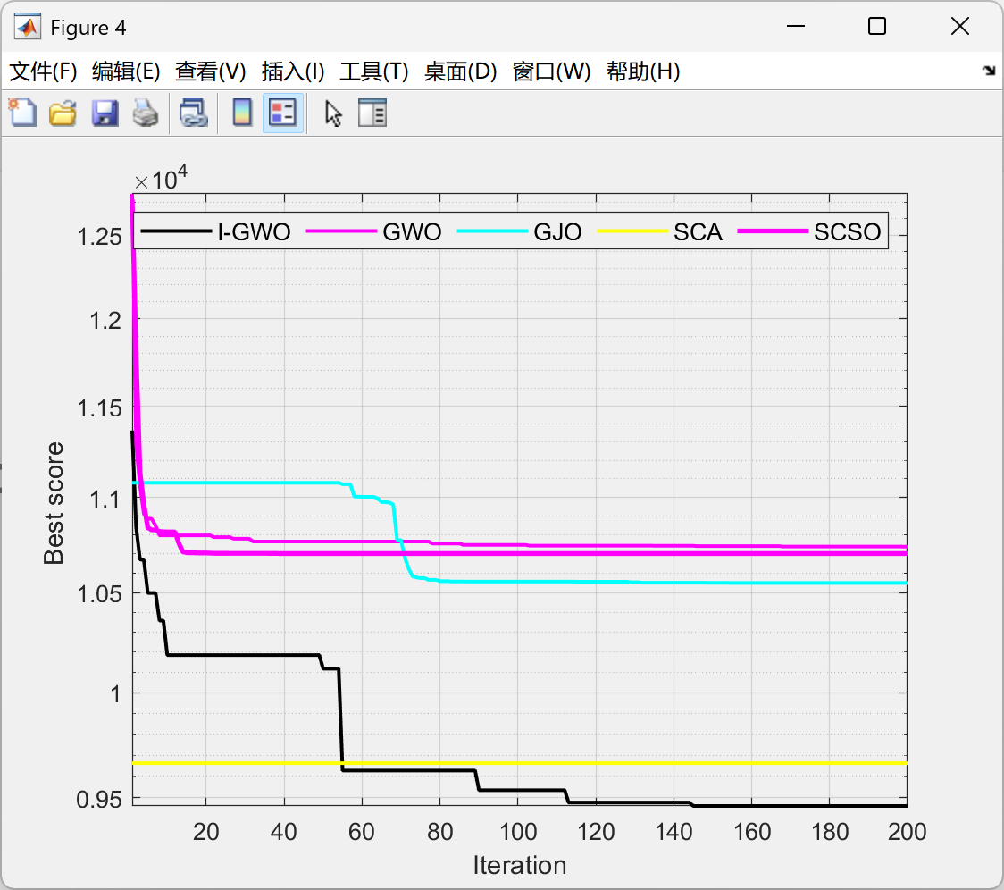AI Visual Insight: This figure shows UAV trajectory distributions over complex 3D mountain terrain. You can typically observe the start and goal positions, the locations of threat zones, and the obstacle avoidance trends of the trajectories. If a path hugs ridgelines or contains sharp bends, its smoothness is likely poor. If the trajectory remains continuous and keeps a safe margin from threat zones, the algorithm has likely achieved a better balance between safety and path length.

AI Visual Insight: This figure most likely corresponds to a convergence curve comparison across algorithms. If the I-GWO curve drops faster in the early stage and continues decreasing in the later stage, it suggests that the nonlinear convergence factor and adaptive perturbation effectively delay premature convergence while preserving final optimization accuracy.

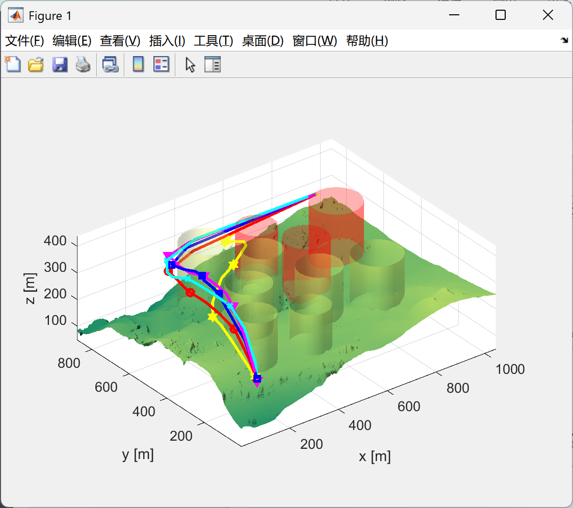
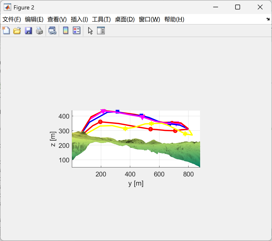AI Visual Insight: This figure most likely presents the final trajectories of multiple algorithms or local obstacle avoidance details. If the path contains gentler turning angles and more uniform altitude changes, it indicates that the spherical coordinate representation and smoothness penalty term directly improve trajectory flyability.

AI Visual Insight: This figure may be a box plot, bar chart, or statistical indicator plot used to show the mean, best value, and variation range across 30 runs. If the I-GWO distribution is more concentrated and its median is lower, that directly indicates stronger robustness than the other candidate algorithms.

Based on the original description, I-GWO generates shorter trajectories, smoother turns, and safer obstacle avoidance margins. This means its advantage appears not only in numerical fitness, but also in the geometric path quality that can directly benefit the flight control layer.

The engineering value of this work lies in its unified modeling, optimization, and evaluation pipeline

The real value of this study is not just the proposal of an improved Grey Wolf algorithm, but the establishment of a complete technical loop: terrain modeling, threat modeling, spherical coordinate trajectory representation, composite cost design, multi-algorithm comparison, and statistical experimental validation. That makes it more like a transferable path planning experiment template.

If future work integrates dynamic obstacle perception, online replanning, and multi-UAV coordination, this framework remains extensible. In particular, for low-altitude logistics, mountain inspection, and emergency search-and-rescue missions, I-GWO-style algorithms that emphasize stability and flyability offer stronger application potential.

FAQ

Why are intelligent optimization algorithms better suited to UAV 3D path planning?

Because the problem simultaneously includes terrain, threat, altitude, and smoothness constraints, the objective space is usually non-convex and non-differentiable. Intelligent optimization algorithms do not rely on gradients and can optimize directly in complex search spaces.

What are the core improvements of I-GWO over standard GWO?

The core improvements are threefold: a nonlinear convergence factor for better search rhythm control, adaptive perturbation for stronger local exploitation, and Cauchy mutation for improved ability to escape local optima. Together, they improve convergence speed, accuracy, and stability.

What practical value do spherical coordinates provide in this type of path planning?

They reduce redundancy in the search variables, represent heading and pitch changes more naturally, and make it easier to directly constrain turn angles and climb angles. As a result, they produce smoother, more executable trajectories that better match UAV dynamics.

Core Summary

This article reconstructs a UAV 3D trajectory planning study based on GWO, I-GWO, GJO, SCSO, and SCA. It focuses on complex mountain environment modeling, spherical coordinate trajectory representation, a multi-objective cost function, and the three improvement strategies in I-GWO, then uses Matlab simulation results to analyze differences in convergence speed, stability, and path quality.