This article focuses on improving the accuracy of 3D vision robot hand-eye calibration: first, use the traditional AX=XB formulation to obtain the initial extrinsic parameters from the camera to the robot base, then apply ICP to perform rigid registration on corresponding corner-point sets for secondary refinement. This approach addresses the accuracy ceiling imposed by the number of poses and sampling quality in the initial calibration stage. Keywords: hand-eye calibration, ICP, 3D vision.
Technical specification snapshot
| Parameter | Details |
|---|---|
| Domain | 3D vision robot hand-eye calibration |
| Core algorithms | point-to-point ICP, AX=XB |
| Implementation languages | C++ / Python |
| Common libraries | OpenCV, PCL, Eigen |
| Transformation type | 3D rigid transformation SE(3) |
| Input data | T_board_to_cam, robot poses, 3D corner coordinates |
| Protocols / data interfaces | Camera SDK, robot controller TCP / teach pendant readings |
| Star count | Not provided in the original article |
| Core dependencies | PCL ICP, SVD, calibration board corner extraction |
ICP is well suited as a secondary refinement step after hand-eye calibration
Traditional hand-eye calibration typically starts by fixing the calibration board, then collecting multiple robot poses and their corresponding images, and finally solving AX=XB to estimate the camera-to-base extrinsic matrix T_cam_to_base. This step produces usable results, but its accuracy ceiling is jointly constrained by pose distribution, pose count, and corner quality.
In a 3D camera setup, each checkerboard corner provides not only pixel coordinates but also 3D coordinates in the camera frame. As a result, the same physical point can be observed in both the camera frame and the robot base frame. That makes rigid registration possible.
The goal of point-to-point ICP is to minimize the sum of squared distances between corresponding points
The essence of point-to-point ICP is straightforward: given two sets of corresponding points, solve for the rotation matrix R and translation vector t so that the transformed source point cloud aligns as closely as possible with the target point cloud. It assumes there is no scale difference between the two datasets, only rigid motion.
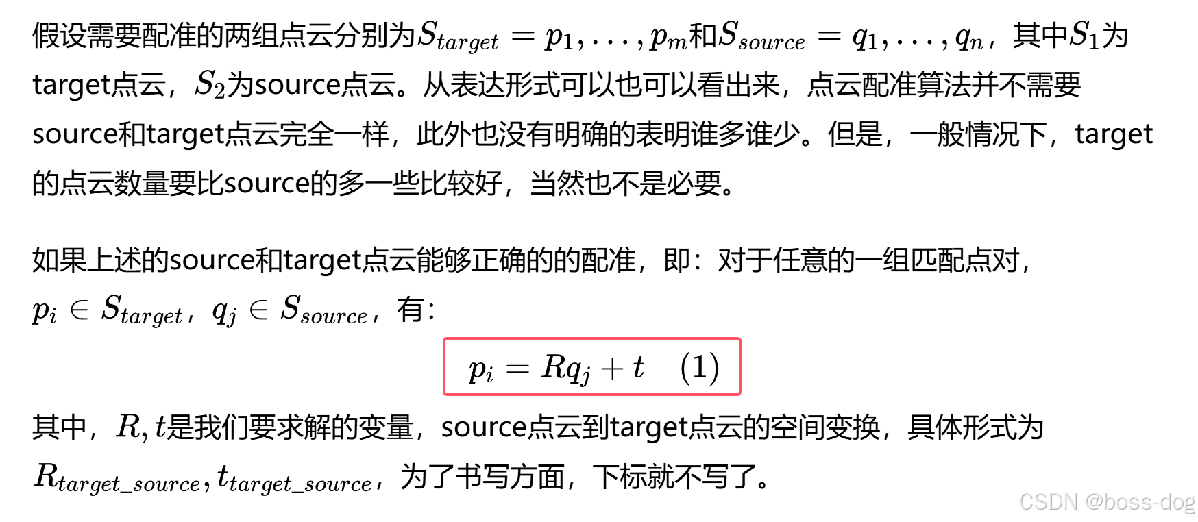 AI Visual Insight: This image illustrates the optimization objective of ICP. Given known point correspondences, the algorithm solves for rotation and translation to minimize the sum of squared Euclidean distances between two sets of 3D points. This objective is typically formulated as a least-squares problem and serves as the mathematical foundation for refining extrinsic parameters after hand-eye calibration.
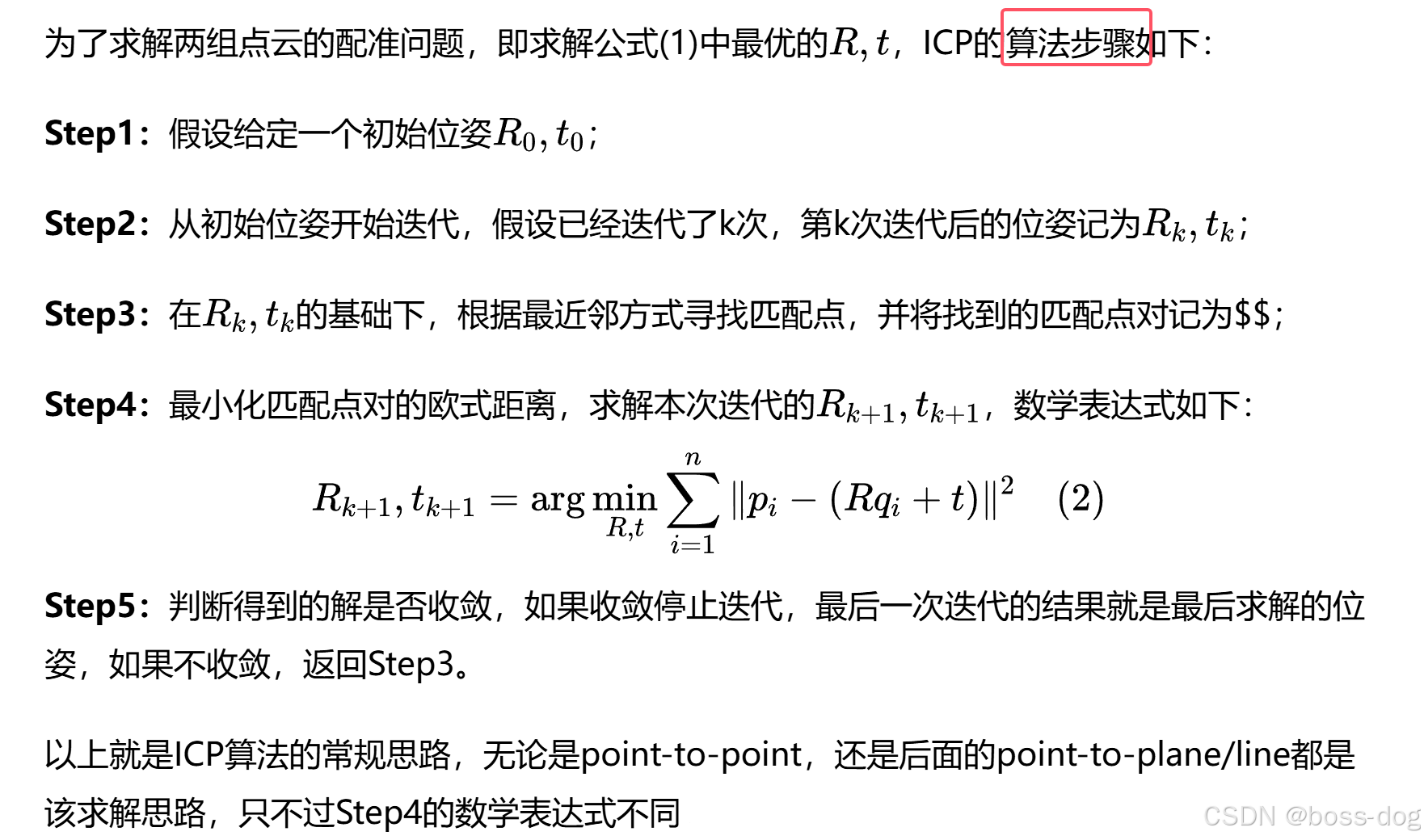 AI Visual Insight: This image shows the standard iterative flow of ICP: initialize the pose, search for nearest-neighbor correspondences, compute the current transformation, update the error, and check for convergence. It highlights that ICP depends heavily on the quality of the initial estimate, which is why it is better used as a local optimizer after hand-eye calibration rather than as a global solver from scratch.
import numpy as np

def solve_rigid_transform(cam_pts, base_pts):
    # Compute the centroids of the two point sets
    c1 = cam_pts.mean(axis=0)
    c2 = base_pts.mean(axis=0)

    # Remove centroids and preserve only the rigid rotation-translation relationship
    q1 = cam_pts - c1
    q2 = base_pts - c2

    # Build the covariance matrix
    H = q1.T @ q2
    U, S, Vt = np.linalg.svd(H)

    # Solve the rotation matrix with SVD
    R = Vt.T @ U.T
    if np.linalg.det(R) < 0:  # Prevent a reflection matrix
        Vt[-1, :] *= -1
        R = Vt.T @ U.T

    # Solve the translation vector from the centroid relationship
    t = c2 - R @ c1
    return R, t
This code demonstrates the core process of solving a rigid transformation with SVD in point-to-point registration.
The key value of ICP lies in local refinement based on the initial extrinsics
The strength of ICP is that it directly optimizes the rigid relationship between two sets of 3D points, but it is sensitive to the initial pose. If the initial estimate deviates too much, the algorithm can easily converge to a local optimum and produce an incorrect result.
For that reason, the more robust engineering path is not to replace hand-eye calibration with ICP, but to perform hand-eye calibration first and then apply ICP for correction. AX=XB provides an initial estimate close to the ground truth, and ICP then compresses the residual error. That is the core idea behind this workflow.
In an eye-to-hand setup, the data can be clearly organized into three groups
The first group consists of T_board_to_cam under multiple poses, which is used by OpenCV or similar tools to solve the initial T_cam_to_base. The second group is the checkerboard corner 3D coordinates measured directly by the camera, denoted as cam_Pi. The third group is base_Pi, recorded in the robot base frame after the robot tool tip touches each corner point one by one.
As long as cam_Pi and base_Pi represent the same set of physical corner points, you can feed these two point sets into ICP. The optimization target is: base_Pi = T * cam_Pi. Here, T is the compensation applied to the initial hand-eye extrinsics.
#include <pcl/registration/icp.h>
#include <pcl/point_types.h>
#include <pcl/point_cloud.h>

using PointT = pcl::PointXYZ;

pcl::IterativeClosestPoint<PointT, PointT> icp;
// source: corner points in the camera coordinate system
icp.setInputSource(cam_cloud);
// target: corner points in the robot base coordinate system
icp.setInputTarget(base_cloud);

// Set iteration parameters to control convergence behavior
icp.setMaximumIterations(50);
icp.setMaxCorrespondenceDistance(0.01);  // The unit is typically meters
icp.setTransformationEpsilon(1e-8);

pcl::PointCloud
<PointT> aligned;
// Use the initial extrinsics as the starting estimate for iterative refinement
icp.align(aligned, init_T_cam_to_base);

Eigen::Matrix4f refined_T = icp.getFinalTransformation();
This code shows how to use the initial hand-eye calibration result as the ICP starting estimate in PCL for secondary registration refinement.
Improving accuracy depends not only on the algorithm but also on data quality
Whether ICP can actually improve accuracy depends on whether the point correspondences are accurate enough. If the camera-side corner 3D coordinates suffer from significant depth noise, or if the robot-side TCP is not calibrated precisely, those errors will be injected directly into the optimization.
Point distribution also matters. If all points are concentrated in a local region, even a large number of points may still provide insufficient rotational constraints. A better approach is to choose corner points that cover a larger area and maximize the geometric baseline whenever possible.
Whether three points are enough depends on mathematical solvability versus engineering robustness
In theory, three non-collinear point pairs are sufficient to determine a 3D rigid transformation. In practice, however, using only three points often provides poor noise robustness and is highly sensitive to probing errors and depth errors.
A better recommendation is to collect at least 6 to 12 well-distributed corner points, then evaluate the ICP convergence error, mean residual, and repeatability across multiple experiments. If you must reduce robot teaching time, prioritize the checkerboard corners and representative points near the center.
def update_handeye(T_init, T_icp):
    # ICP outputs the compensation or refined transform from camera frame to base frame
    # Update the final extrinsics by left-multiplication
    return T_icp @ T_init
This code summarizes the final extrinsic update rule, using the ICP result to refine the initial hand-eye matrix.
This workflow is well suited for high-precision grasping and offline compensation scenarios
When a robot performs high-precision insertion, grasping, or localization tasks, traditional hand-eye calibration often exposes millimeter-level errors. If the system already includes a 3D camera and supports robot teaching, adding ICP as an offline compensation step is usually more cost-effective than redoing the entire calibration pipeline.
Keep in mind that ICP can only correct rigid transformation errors. It cannot replace camera intrinsic calibration, TCP calibration, or robot body error compensation. If the error originates from systematic distortion, ICP alone will not solve the root problem.
FAQ structured Q&A
Q1: Why not use ICP directly for hand-eye calibration instead of doing AX=XB first?
A: Because ICP is sensitive to the initial pose. If the starting estimate is poor, it can easily get trapped in a local optimum. AX=XB first provides extrinsics close to the true solution, and ICP is better suited for local refinement on top of that estimate.
Q2: How should you choose between point-to-point and point-to-plane here?
A: If the input consists of discrete feature points such as checkerboard corners, point-to-point is more direct. If the input is a high-quality dense planar point cloud, point-to-plane often converges faster and can achieve higher accuracy.
Q3: Is the refined matrix always more accurate after ICP optimization?
A: Not necessarily. ICP can improve accuracy only when the point correspondences are accurate, the initial estimate is reasonable, and the point distribution is good. If depth noise is high, probing error is large, or the point count is too small, the result can actually become worse.
Core summary
This article reconstructs an engineering workflow for improving 3D vision robot hand-eye calibration accuracy with ICP. The process first uses AX=XB to estimate the initial camera-to-base transform, then performs rigid registration between corresponding corner points in the camera coordinate system and the robot base coordinate system, and finally outputs a correction matrix to refine T_cam_to_base. The discussion covers point-to-point ICP principles, data collection, PCL implementation ideas, and practical deployment considerations.