Multi-UAV Distributed Cooperative Path Planning and Collision Avoidance in MATLAB: APF Simulation Framework for Dynamic 3D Environments

A multi-UAV cooperative path planning system for dynamic 3D environments, built in MATLAB with a distributed simulation framework. It combines the Artificial Potential Field (APF) method, dynamic obstacle updates, and inter-UAV collision avoidance to address real-time planning and safe deconfliction in swarm flight. Keywords: multi-UAV, path planning, collision avoidance.

Technical Specifications Snapshot

Parameter	Description
Primary Language	MATLAB
System Type	Multi-UAV distributed cooperative planning simulation
Core Protocols / Mechanisms	Artificial Potential Field (APF), Velocity Obstacle (VO), priority-based collision avoidance
Simulation Scenario	100m × 100m × 50m 3D space
Number of UAVs	5
Obstacle Configuration	8 static obstacles, 3 dynamic obstacles
Safety Distance	5m
Simulation Time Step	0.1s
Maximum Iterations	500
Core Dependencies	MATLAB base computation and plotting capabilities
Stars	Not provided in the original input

The system targets the core challenge of multi-UAV cooperative planning in dynamic environments

The central challenge in multi-UAV systems is not simply finding a path for one vehicle. It is ensuring arrival efficiency, obstacle avoidance safety, and cooperative stability at the same time within a shared airspace. The original implementation uses a representative simulation task with five UAVs operating in a dynamic 3D environment.

Its objective is straightforward: multiple UAVs start from different initial positions, navigate in the presence of static and moving obstacles, reach their respective target points, and avoid inter-UAV collisions throughout the mission. This problem maps directly to real-world scenarios such as search and rescue, inspection, surveying, and formation logistics flight.

AI Visual Insight: This image functions more like a project cover or thematic illustration. It emphasizes the topic of multi-UAV cooperative path planning and collision avoidance, typically serving as a scenario-level visual introduction rather than a direct algorithm output.

The system uses a layered force-field model to organize planning logic

This implementation is essentially a local real-time planner. At each simulation step, every UAV independently computes three types of forces: target attraction, obstacle repulsion, and inter-UAV collision avoidance. The planner then sums these components into a total force, which updates velocity and position.

The value of this design lies in its structural clarity, direct computation, and strong real-time behavior. For small- to medium-scale UAV swarms, it is especially well suited for quickly validating whether a cooperative strategy works.

num_uav = 5;                 % Number of UAVs
safe_dist = 5.0;             % Inter-UAV safety distance
obs_dist = 3.0;              % Obstacle safety distance
dt = 0.1;                    % Simulation time step
max_iter = 500;              % Maximum number of iterations
max_vel = 10.0;              % Maximum velocity

uav_pos = start_pos;         % Initialize positions
uav_vel = zeros(num_uav,3);  % Initialize velocities

This code block defines the basic constraints of the cooperative simulation and serves as the parameter entry point for the entire planning loop.

The simulation results confirm that the collision avoidance strategy is practically usable

The original results present four key outputs: 3D trajectories, minimum-distance curves, velocity and acceleration profiles, and distance-to-goal convergence. Together, these plots are sufficient to assess whether the algorithm can run, avoid collisions, and converge.

AI Visual Insight: This figure provides an overall view of the simulation results. It typically includes multi-UAV paths, obstacle locations, and target distributions, making it useful for quickly judging trajectory intersections, mission convergence, and spatial efficiency in a dynamic environment.

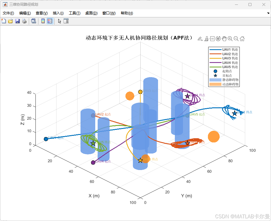AI Visual Insight: This 3D trajectory plot distinguishes each UAV path with a different color. It allows direct observation of start and end point distribution, obstacle bypass behavior, and the degree of trajectory separation during cooperative flight. It is a core visualization for evaluating planning feasibility and obstacle avoidance effectiveness.

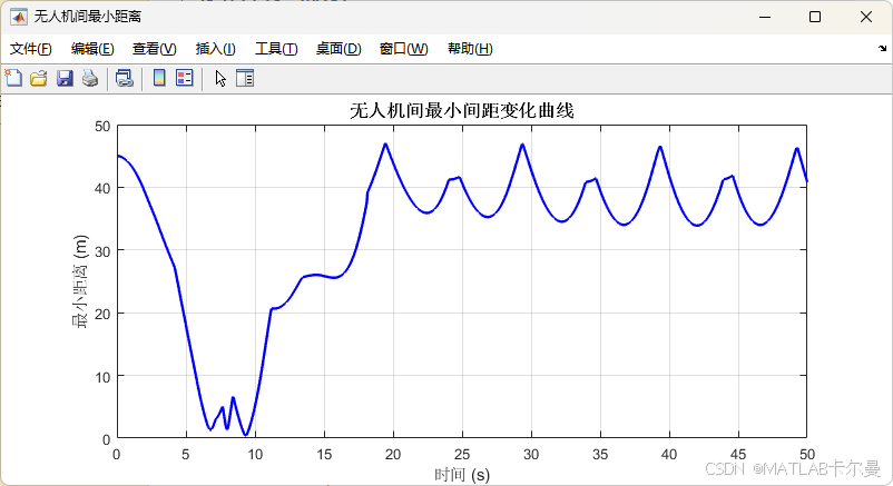AI Visual Insight: This curve shows how the minimum distance between UAVs changes over time. If the curve stays consistently above the 5 m safety threshold, it indicates that the collision prediction and avoidance-force model effectively suppress near-range risk during dynamic cooperation.

Velocity smoothness and convergence are key indicators of engineering value

Even if a path avoids obstacles, the algorithm is still unsuitable for real flight control systems if velocity fluctuates violently. The original results note that both velocity and acceleration change smoothly. That indicates the force superposition and saturation mechanisms do not introduce significant numerical oscillation.

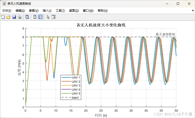AI Visual Insight: This figure shows the time-series behavior of velocity or acceleration. If the curves remain continuous without high-frequency spikes, the position update and velocity saturation strategies are relatively stable and better aligned with UAV dynamic constraints and smooth actuator control requirements.

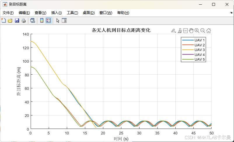AI Visual Insight: This convergence plot tracks how each UAV’s distance to its goal decays over time. If the curves generally decrease monotonically and eventually approach zero, the attractive and avoidance terms are well balanced and do not become trapped in long-term local oscillation.

for iter = 1:max_iter
    dynamic_obs = update_dynamic_obs(dynamic_obs, dt); % Update dynamic obstacles
    all_obs = [static_obs; dynamic_obs];               % Merge obstacle sets

    for i = 1:num_uav
        F_att = compute_attractive_force(uav_pos(i,:), goal_pos(i,:)); % Target attraction force
        F_rep = compute_repulsive_force(uav_pos(i,:), all_obs, obs_dist); % Obstacle repulsive force
        F_col = compute_collision_avoidance(i, uav_pos, safe_dist); % Inter-UAV collision avoidance force

        F_total = F_att + F_rep + F_col;              % Sum total force
        uav_vel(i,:) = uav_vel(i,:) + F_total * dt;   % Update velocity
        uav_pos(i,:) = uav_pos(i,:) + uav_vel(i,:) * dt; % Update position
    end
end

This main loop implements dynamic obstacle updates, distributed force computation, and UAV state propagation.

The core algorithm consists of attraction, repulsion, and predictive collision avoidance

The attractive force pulls each UAV toward its target. The repulsive force pushes it away from obstacles. The collision avoidance force handles interactions between UAVs. Combined together, these components give the system both mission direction and safety constraints.

The most notable part is the inter-UAV avoidance term. The original content mentions a Velocity Obstacle (VO) model and a priority mechanism. That means the algorithm does not wait for a collision to happen before reacting. Instead, it predicts conflict windows in advance based on relative velocity, which is much closer to engineering-grade practice.

Modular function decomposition improves replaceability and extensibility

The original design separates static obstacle initialization, dynamic obstacle updates, attractive force computation, repulsive force computation, and collision avoidance into independent functions. This structure is highly suitable for later replacing local methods. For example, you could use RRT* to generate a global guidance path and let APF handle terminal real-time correction.

if vel_norm > max_vel
    uav_vel(i,:) = uav_vel(i,:) / vel_norm * max_vel; % Velocity saturation to prevent unstable divergence
end

if all(vecnorm(uav_pos - goal_pos, 2, 2) < 1.0)
    fprintf('所有无人机已到达目标！\n'); % Termination condition satisfied
    break;
end

This code block ensures numerical stability and closed-loop convergence through velocity saturation and mission completion checks.

The approach works well as a foundation for teaching simulations and algorithm prototyping

From an engineering perspective, this MATLAB implementation is better suited for research validation than direct deployment on physical UAVs. The main reason is that APF is prone to local minima, which can cause stalled obstacle bypassing or non-optimal paths in complex environments.

Its strengths are equally clear: it is easy to implement, easy to explain, easy to tune, and easy to visualize. For course projects, paper prototypes, introductory path planning, and multi-agent cooperative simulation, it is a highly efficient starting point.

The system can evolve further along three practical directions

The first path is to add a global planner such as A, RRT, or hybrid graph search to reduce local optima. The second is to introduce MPC or reinforcement learning to improve predictive control under dynamic constraints. The third is to integrate ROS, PX4, or AirSim to migrate from a MATLAB prototype to software-in-the-loop or semi-physical simulation.

FAQ

1. What is the core algorithm in this multi-UAV path planning code?

The core method is the Artificial Potential Field (APF), combined with dynamic obstacle repulsion and an inter-UAV collision avoidance mechanism based on Velocity Obstacle concepts. Its strengths are strong real-time performance and implementation simplicity, which make it suitable for simulation validation.

2. Why is the minimum-distance curve more important than only looking at 3D trajectories?

A 3D trajectory only shows whether paths appear to intersect visually. It does not quantify safety. The minimum-distance curve directly verifies whether UAVs always remain above the safety threshold, making it a key metric for evaluating whether the collision avoidance strategy is effective.

3. If I want to use this system in more complex scenarios, what should I improve first?

Start by adding a hybrid global-local planning architecture. Use A or RRT to provide a feasible corridor first, then let APF or MPC handle local obstacle avoidance. This can significantly reduce the risk of local minima and oscillation.

AI Readability Summary: This article reconstructs a distributed cooperative path planning approach for multiple UAVs in dynamic 3D environments. It focuses on MATLAB simulation, the Artificial Potential Field method, dynamic obstacle updates, and inter-UAV collision avoidance, while extracting the key parameters, code structure, result interpretation, and future extension paths.