Decision Tree Algorithms Explained: ID3, C4.5, CART, Pruning, and sklearn in Practice

Decision trees are highly interpretable supervised learning algorithms. Their core capability is to perform classification or regression through feature-based splits. They address two common challenges: poor model interpretability and unclear feature selection logic. The key topics include ID3, C4.5, and CART. Keywords: Decision Tree, Information Gain, Gini Impurity.

Technical Specification Snapshot

Parameter	Details
Language	Python
Task Type	Classification, Regression
Core Algorithms	ID3, C4.5, CART
Common Implementation	scikit-learn
Feature Selection Metrics	Information Gain, Gain Ratio, Gini Impurity
Typical Pain Points	Overfitting, continuous feature splitting, interpretability trade-offs

Decision trees split data with rule-based logic in supervised learning

A decision tree essentially converts if-else logic into a tree structure. Internal nodes represent feature-based decisions, branches represent decision outcomes, and leaf nodes represent the final class or numeric prediction. Its greatest strength is not maximum accuracy, but transparent rules and easy interpretation.

The standard training workflow has three steps: select the best feature, recursively grow subtrees, and prune when necessary. If you do not constrain tree depth, the model will continue fitting fine-grained details in the training set and eventually overfit.

A minimal training example immediately shows the interpretability of a decision tree

from sklearn.tree import DecisionTreeClassifier
from sklearn.model_selection import train_test_split
from sklearn.datasets import load_iris

# Load the Iris dataset
X, y = load_iris(return_X_y=True)

# Split the training set and test set
X_train, X_test, y_train, y_test = train_test_split(
    X, y, test_size=0.2, random_state=42
)

# Train a classification tree with Gini impurity
model = DecisionTreeClassifier(criterion="gini", max_depth=3, random_state=42)
model.fit(X_train, y_train)  # Core logic: fit the decision tree

print(model.score(X_test, y_test))  # Output test set accuracy

This code shows how to quickly train an interpretable classification tree with sklearn.

ID3 selects the feature that reduces uncertainty the most through information gain

The core of ID3 is information entropy. Entropy measures the uncertainty of a dataset. The more evenly distributed the classes are, the higher the entropy; the purer the classes are, the lower the entropy. When a feature significantly reduces disorder after splitting, it becomes a stronger candidate for the current split.

Information gain is defined as the entropy before splitting minus the conditional entropy after splitting on a feature. The larger the gain, the more certainty the feature provides, so the higher its priority. ID3 is useful for understanding why one feature should be chosen before another.

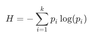AI Visual Insight: The image presents the mathematical definition of information entropy and highlights that entropy increases as the class probability distribution becomes more uniform. It serves as the theoretical starting point for conditional entropy and information gain.

Writing the entropy function by hand helps clarify the basis of feature selection

import math
from collections import Counter

def entropy(labels):
    total = len(labels)
    counter = Counter(labels)
    ent = 0.0
    for count in counter.values():
        p = count / total
        ent -= p * math.log2(p)  # Core logic: accumulate uncertainty using the entropy formula
    return ent

print(entropy(["yes", "yes", "no", "no", "yes"]))

This code computes the entropy of a label set and provides the shortest path to understanding ID3.

C4.5 fixes ID3’s preference for high-cardinality features with gain ratio

A typical weakness of ID3 is that it favors features with many distinct values. For example, a user ID can almost separate every sample individually, producing extremely pure splits but offering almost no generalization value. Such features may look excellent on the training set while creating meaningless splits in practice.

C4.5 addresses this issue with gain ratio. It adds a penalty term based on the split information of the feature itself. The more distinct values a feature has, the larger the penalty, which suppresses the illusion of high-value multi-valued features.

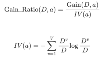AI Visual Insight: The image emphasizes the structure of Gain Ratio = IG / IV(A), where IV(A) acts as a penalty term that directly reflects the complexity of a feature’s value distribution. This is the key design improvement that makes C4.5 stronger than ID3.

The three mainstream decision tree algorithms use different feature selection criteria

Algorithm	Selection Metric	Applicable Tasks	Main Characteristics
ID3	Information Gain	Classification	Simple and intuitive, but biased toward high-cardinality features
C4.5	Gain Ratio	Classification	Reduces multi-value bias and can handle continuous attributes
CART	Gini Impurity / MSE	Classification, Regression	Binary tree structure and the most common engineering implementation

This comparison table works well as a quick reference for interviews and model selection.

CART is more common in production because it supports both classification and regression

CART classification trees no longer use entropy. Instead, they use Gini impurity. The smaller the Gini value, the purer the node, so the algorithm searches for the feature and split point that minimize the weighted Gini impurity after splitting. Compared with ID3 and C4.5, CART is often more direct computationally.

For regression tasks, CART switches to squared error minimization. It splits continuous-value samples into two groups using candidate thresholds, compares the total loss after different splits, and selects the threshold with the smallest error. Each leaf node outputs the mean value of samples in that region.

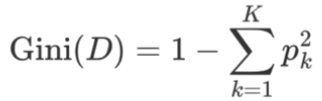AI Visual Insight: The image shows the core Gini impurity formula and explains that node purity can be derived from the sum of squared class probabilities. When one class probability approaches 1, the Gini value approaches 0.

sklearn uses a CART-style classification tree by default

from sklearn.tree import DecisionTreeClassifier

# criterion="gini" means Gini impurity is used
clf = DecisionTreeClassifier(
    criterion="gini",
    max_depth=5,          # Core logic: limit tree depth to reduce overfitting
    min_samples_split=10, # Core logic: stop splitting when a node has too few samples
    min_samples_leaf=5,
    random_state=42
)

This parameter setup reflects the basic way CART is controlled in real projects.

Decision trees show strong interpretability in Titanic survival prediction

In the Titanic use case, the input features usually include passenger class, age, sex, fare, and port of embarkation. Decision trees do not require feature scaling, and they handle categorical variables intuitively, which makes them excellent as both a first baseline model and a business-facing explanation model.

A typical workflow includes imputing missing values, encoding categories, splitting the training and test sets, training the decision tree, and tuning depth and leaf size. If the goal is to explain who is more likely to survive, a decision tree usually has a stronger communication advantage than a black-box model.

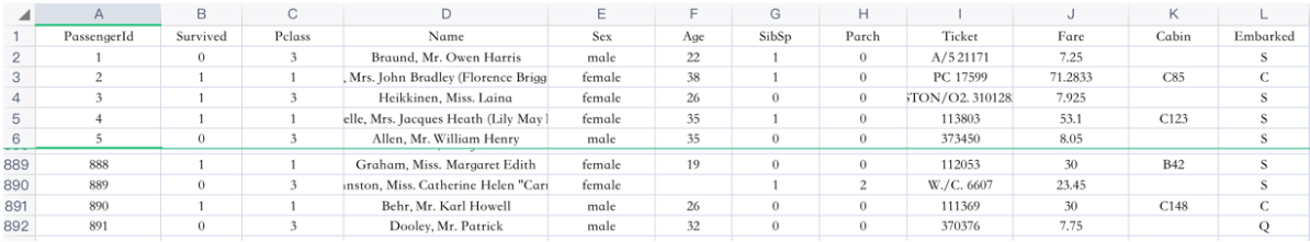AI Visual Insight: The image shows the field structure of the Titanic dataset and illustrates that decision trees can directly split on mixed discrete and continuous features, which makes this dataset a classic teaching and beginner-friendly practice example.

A simplified end-to-end workflow is enough to serve as a project scaffold

import pandas as pd
from sklearn.model_selection import train_test_split
from sklearn.tree import DecisionTreeClassifier

# Load the dataset and build basic features
train = pd.read_csv("train.csv")
train["Age"] = train["Age"].fillna(train["Age"].mean())  # Core logic: fill missing age values
train["Sex"] = train["Sex"].map({"male": 0, "female": 1})

X = train[["Pclass", "Age", "Sex", "SibSp", "Parch", "Fare"]]
y = train["Survived"]

X_train, X_test, y_train, y_test = train_test_split(X, y, random_state=42)
model = DecisionTreeClassifier(max_depth=4, random_state=42)
model.fit(X_train, y_train)  # Core logic: train the survival prediction tree

This code provides a minimal runnable path from tabular data to a tree-based model.

Pruning is the key to controlling overfitting, not improving training-set accuracy

Tree models have strong fitting capacity. Especially when the sample size is small, features are noisy, or the data contains many irregular patterns, the model can learn accidental structure as well. The goal of pruning is to actively remove low-value branches and improve generalization, not to keep reducing training error.

Pre-pruning stops tree growth early during construction, for example by limiting maximum depth or the minimum number of samples required for a split. Post-pruning first grows a full tree and then removes subtrees bottom-up if they do not improve validation performance. The former is faster, while the latter often generalizes more reliably.

Common pruning parameters are essentially pre-pruning strategies

from sklearn.tree import DecisionTreeRegressor

reg = DecisionTreeRegressor(
    max_depth=3,          # Core logic: limit tree depth
    min_samples_split=8,  # Core logic: constrain further splitting
    min_samples_leaf=4,
    random_state=42
)

This code shows that in most engineering scenarios, pruning starts with hyperparameter constraints.

FAQ provides structured answers to common questions

Q1: How can you quickly distinguish ID3, C4.5, and CART?

A: ID3 uses information gain, C4.5 uses gain ratio, and CART uses Gini impurity or squared error. In production, CART is the most common because it supports both classification and regression and has mature implementations.

Q2: Why do decision trees overfit so easily?

A: Because a tree keeps splitting until nodes become sufficiently pure, it can memorize noise and accidental patterns in the training set. Common solutions include limiting max_depth, increasing min_samples_leaf, applying pruning, or using ensemble learning.

Q3: When should you prioritize decision trees?

A: Decision trees are an excellent starting point when the task emphasizes rule interpretability, nonlinear feature relationships, and minimal preprocessing or normalization. If you need stronger generalization, you typically move on to Random Forests or Gradient Boosted Trees.

Core Summary: This article systematically reconstructs the core knowledge of decision trees, covering information gain in ID3, gain ratio in C4.5, Gini impurity and regression tree principles in CART, and practical sklearn entry points. It helps developers quickly build interpretable classification and regression models.