Underwater Robot Dual-Manipulator Dynamic Modeling and Control Simulation: Methods, Models, and Matlab Implementation - Devuly | Smart Analytics for Developers & Projects

This article focuses on dynamic modeling and control simulation for an underwater robot dual-manipulator system. It covers multibody dynamics, hydrodynamic drag and added-mass compensation, coordinated dual-arm control, and Matlab implementation approaches. The goal is to address strong underwater nonlinearities, large disturbances, and the challenges of dual-arm coordination. Keywords: underwater robots, dual manipulators, Matlab simulation.

Table of Contents

Technical Specifications Snapshot

Parameter	Description
Primary Language	Matlab
Modeling Methods	Lagrangian method, Newton-Euler method
Control Target	Underwater robot dual-manipulator system
Environmental Characteristics	Hydrodynamic drag, added mass, hydrodynamic disturbances
Control Strategies	PID, fuzzy control, neural network control, coordinated control
Protocols/Interfaces	Not explicitly specified; primarily a Matlab simulation workflow
Stars	Not provided
Core Dependencies	Matlab, Control System Toolbox, numerical computing modules

The value of underwater dual-manipulator systems lies in improving complex task capability

Underwater robots are widely used in ocean exploration, engineering maintenance, and sample collection. A single manipulator struggles to complete composite tasks such as grasping, assembly, and cooperative handling. For that reason, dual manipulators have become a key configuration for improving operational efficiency and manipulation freedom.

The real challenge is not simply making the manipulators move. It is enabling them to perform stable, high-precision operations under underwater disturbances, communication delays, and constrained spaces. This directly determines the upper bound of both modeling accuracy and control strategy performance.

The underwater environment imposes stronger constraints on control systems

First, manipulator motion in water experiences significant drag, and that drag is usually velocity-dependent. Compared with operation in air, hydrodynamic effects make the system substantially more nonlinear and more strongly coupled.

Second, the added-mass effect changes the equivalent inertia parameters. When the manipulators accelerate or decelerate, they must overcome not only their own inertia but also the surrounding fluid they displace. This makes the dynamic equations fundamentally different from those of land-based robotic arms.

Third, the dual-arm workspace is often constrained. For tasks such as pipeline connection, valve operation, or sample grasping, the system must also handle collision avoidance, trajectory synchronization, and end-effector force coordination.

Dynamic modeling must cover rigid-body, fluid, and joint-level behavior

Multibody dynamics form the foundation of the entire system model. A dual-manipulator system can be abstracted as a serial-parallel structure composed of multiple links and joints, then coupled with the underwater platform to form an overall dynamic model.

When using the Lagrangian method, engineers typically derive the equations from the system’s kinetic and potential energy. This approach is well suited to a unified expression of generalized-coordinate dynamics for complex systems. If force analysis and recursive computation are more important, the Newton-Euler method is often more practical from an engineering perspective.

% Define joint states
q  = [q1;q2;q3;q4];          % Joint angles
qd = [dq1;dq2;dq3;dq4];      % Joint angular velocities
qdd = [ddq1;ddq2;ddq3;ddq4]; % Joint angular accelerations

% Build dynamic terms
M = calcInertia(q);          % Compute inertia matrix
C = calcCoriolis(q, qd);     % Compute Coriolis and centrifugal terms
G = calcGravity(q);          % Compute gravity and buoyancy terms
D = calcHydroDrag(qd);       % Compute hydrodynamic drag term

% System dynamic equation
Tau = M*qdd + C*qd + G + D;  % Output actuator joint torque

This code shows the basic way to organize the dual-manipulator dynamic equations in Matlab.

Hydrodynamic compensation determines whether the model behaves like a real underwater system

In practical engineering, a pure rigid-body model is usually not enough to reproduce actual motion response. The dynamic equations must include hydrodynamic drag, added-mass terms, and random disturbance torques.

Hydrodynamic drag is often approximated using linear or quadratic velocity terms. Added mass can be incorporated into the inertia matrix to build an equivalent mass model that more closely reflects the real environment. For irregular ocean-current disturbances, the simulator can inject them as stochastic processes or bounded disturbances.

function D = calcHydroDrag(qd)
    Cd = diag([1.8,1.5,1.2,1.0]);      % Drag coefficient matrix
    D  = Cd * abs(qd) .* qd;           % Quadratic drag approximation based on velocity
end

This code constructs a simplified nonlinear hydrodynamic drag model, which is useful for quickly validating controller robustness during the tuning phase.

Joint dynamic modeling determines control accuracy and actuator controllability

At the joint level, engineers cannot assume ideal drive torque alone. Friction, elasticity, backlash, and motor characteristics all contribute to tracking error, especially during low-speed precision manipulation and dual-arm coordination.

A common approach is to model Coulomb friction together with viscous friction, then add motor torque constants and gearbox efficiency. If the joints include compliant structures, the model should also include equivalent stiffness and damping terms.

Control simulation must satisfy stability, robustness, and coordination at the same time

Traditional PID control is easy to implement and works well for quick validation in single-joint or weak-disturbance scenarios. In underwater dual-manipulator operations, it can serve as a baseline controller, but it is often not sufficient on its own to handle strong coupling and parameter uncertainty.

As a result, more effective solutions usually adopt either a hybrid design of classical control plus intelligent compensation or a position-control framework with coordination constraints. For example, PID can maintain baseline tracking, while fuzzy rules or a neural network provide online error compensation.

% Desired joint trajectories for both arms
q_ref = trajPlan(t);                    % Trajectory planning output
e     = q_ref - q;                     % Position error
ed    = qd_ref - qd;                   % Velocity error

% PID control law
Tau_c = Kp*e + Ki*int_e + Kd*ed;       % Generate control torque

% Add coordination term to constrain the relative end-effector pose of both arms
Tau   = Tau_c + Ksync*(x_left - x_right); % Dual-arm synchronization control

This control block implements joint tracking together with dual-arm synchronization constraints.

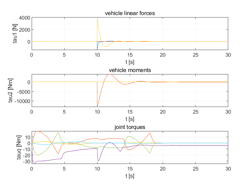
Simulation results are primarily used to validate trajectories, stability, and disturbance rejection

The source material includes several result plots that typically correspond to joint response curves, error convergence, end-effector trajectories, or control input variation. Although the original text does not explain each figure individually, they show that the model can be solved numerically and used to verify closed-loop control performance.

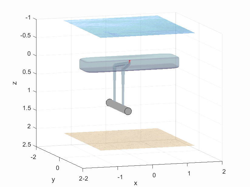
AI Visual Insight: This image shows a simulation output curve window, typically used to compare the desired trajectory with the actual response. If the curves are smooth and converge quickly, the controller likely provides good stability and tracking performance under the current hydrodynamic parameters.

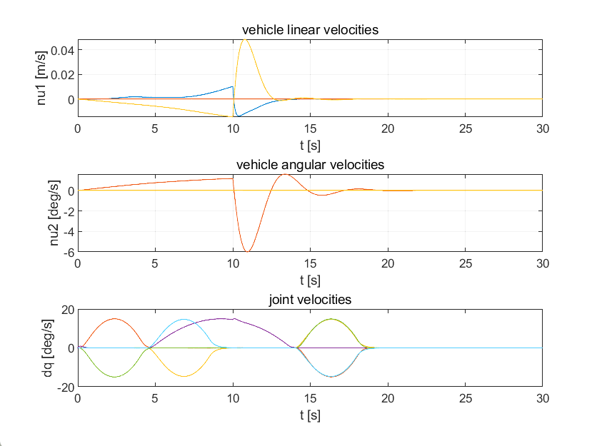
AI Visual Insight: This figure most likely shows state variables or joint angles over time. If the multi-channel curves evolve synchronously without obvious oscillation, that usually indicates the dual-manipulator coordinated control has established effective coupling constraints.

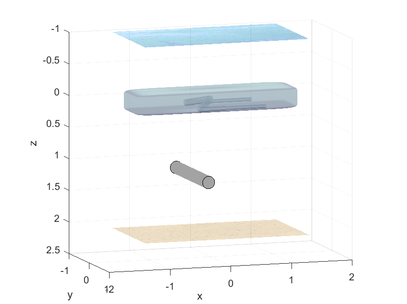
AI Visual Insight: This result plot may correspond to control error, disturbance response, or end-effector trajectory deviation. If the error decays close to zero in a short time, the model compensation and controller tuning are likely well designed.

AI Visual Insight: This figure looks more like an integrated results view used to observe overall dynamic behavior under multivariable coupling. It helps engineers assess whether the system has overshoot, hysteresis, or abrupt control torque changes that could create implementation risks.

Engineering implementation should prioritize three categories of metrics

The first category is trajectory tracking accuracy, including joint error and end-effector position error. The second is control cost, such as peak torque and energy consumption. The third is robustness, meaning stable performance under model-parameter mismatch and external disturbances.

If your goal is research reproduction, start with a simplified model and then gradually add added mass, stochastic disturbances, and joint friction. If your goal is engineering deployment, also include sensor noise, communication delay, and actuator saturation limits.

The references show that this direction has a clear research foundation

You can refer to work by Xie Haibin and Shen Lincheng on coordinated dynamic modeling for underwater robotic systems. This type of literature provides the theoretical basis for underwater multibody system modeling, parameter coupling analysis, and controller design.

FAQ

1. Why is modeling an underwater dual-manipulator system more complex than modeling a land-based robotic arm?

Because the system includes not only multibody coupling but also hydrodynamic drag, added mass, and stochastic hydrodynamic disturbances. These factors significantly change the inertia, damping, and control response.

2. What role is Matlab best suited to play in this kind of simulation?

Matlab is well suited for solving dynamic equations, designing controllers, tuning parameters, and visualizing results. When combined with Simulink, it can also build closed-loop control and disturbance-injection models more efficiently.

3. Which controller should beginners implement first?

It is best to start with PID and build a runnable baseline model for a single joint or a single arm. Then you can gradually add dual-arm synchronization constraints, hydrodynamic compensation, and intelligent control modules. This makes it easier to identify error sources and iterate on the system.

Core Summary: This article reconstructs the dynamic modeling and control simulation framework for an underwater robot dual-manipulator system. It focuses on multibody dynamics, hydrodynamic compensation, joint modeling, and coordinated control strategies, and uses Matlab simulation results to illustrate the key implementation path.