This article reconstructs the core Transformer technology stack: how word embeddings evolved from static vectors to dynamic contextual representations, how MHA, MQA, and GQA balance model quality with KV cache efficiency, how MoE expands capacity through sparse activation, and how the three major Transformer architectures map to different task boundaries. Keywords: Transformer, attention mechanism, MoE.
Technical Specification Snapshot
| Parameter | Details |
|---|---|
| Core Topics | Word embedding evolution, attention variants, MoE, Transformer architecture selection |
| Primary Languages | Python / Mathematical formulas / Markdown |
| Core Protocols | Self-attention, causal masking, Top-k routing |
| Stars | Not provided in the original content |
| Core Dependencies | Transformer, Softmax, FFN, KV Cache, Router |
| Representative Models | BERT, GPT, LLaMA, Qwen, Mixtral |
Word embedding technology has evolved from static lookup tables to contextual representations
Word2Vec and GloVe represent the era of static word vectors. The former learns distributed representations from local context windows, while the latter models statistical relationships using a global co-occurrence matrix. Both are efficient, but each word maps to only one vector, which makes polysemy inherently difficult to handle.
Transformers changed that. They first map tokens into base embeddings, then use stacked self-attention layers to fuse context, allowing a token like “Apple” to produce different hidden states in the context of fruit versus the company. This shift marks a critical leap in modern NLP—from semantic proximity to semantic understanding.
You can understand the differences between the three embedding types through a minimal implementation
# Core difference across three representation types: static lookup vs. dynamic encoding

def static_embedding(token, table):
    return table[token]  # Direct lookup; the same word always gets the same vector

def contextual_embedding(tokens, model):
    x = model.token_embed(tokens)      # Base token vectors
    x = model.position_encode(x)       # Inject positional information
    h = model.transformer_layers(x)    # Dynamically update representations through context
    return h                           # Each position gets a context-aware vector
This code captures the essential difference between static word vectors and Transformer-based dynamic embeddings.
Embedding selection maps directly to resource constraints and task goals
| Dimension | Word2Vec | GloVe | Transformer Dynamic Embeddings |
|---|---|---|---|
| Representation Type | Static | Static | Dynamic |
| Context Modeling | Local window | Global co-occurrence | Full-sequence attention |
| Polysemy Handling | Weak | Weak | Strong |
| Inference Cost | Low | Low | High |
| Typical Use Cases | Lightweight retrieval | Representation learning on small to mid-sized corpora | Understanding and generation tasks |
Multi-head attention has evolved from MHA to deployment-oriented GQA
MHA is the standard multi-head attention mechanism. Each head has independent Q, K, and V projections, which gives it the strongest expressive power. But during decoding, each token must cache the full set of K and V tensors for all heads, so KV cache overhead becomes very large.
MQA takes a different approach: all heads share a single K and V while retaining separate Q projections. This reduces the cache from h copies to 1, significantly improving throughput, but it also reduces representational freedom across heads. GQA sits between the two: it shares K and V by group, striking a more practical balance between quality and efficiency.
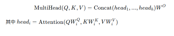 AI Visual Insight: This image illustrates the computation path from standard scaled dot-product attention to concatenated multi-head output. It highlights Q, K, and V linear projections, softmax-based weight normalization, and the structure of parallel heads followed by output projection. It is a key visual for understanding MHA parameter scale and compute flow.
KV cache differences determine large-model deployment cost
# Estimate the number of KV cache units under different attention mechanisms

def kv_cache_units(num_heads, num_groups=None, mode="MHA"):
    if mode == "MHA":
        return num_heads          # Each head caches its own K/V
    if mode == "MQA":
        return 1                  # All heads share one K/V
    if mode == "GQA":
        return num_groups         # Each group shares one K/V
    raise ValueError("unknown mode")
This code shows the fundamental difference in inference memory usage across the three attention variants.
Engineering choices for attention variants follow clear patterns
| Feature | MHA | MQA | GQA |
|---|---|---|---|
| K/V Independence | Per-head independent | Fully shared | Group-shared |
| KV Cache | Largest | Smallest | Medium |
| Inference Speed | Slower | Fastest | Faster |
| Expressive Power | Strongest | Weakest | Best practical trade-off |
| Common Scenarios | Training, smaller models | Extreme inference optimization | Mainstream LLM deployment |
Today’s mainstream large models such as LLaMA, Qwen, and DeepSeek generally favor GQA because it better matches the engineering realities of long-context and high-concurrency inference.
MoE expands model capacity through sparse activation without linearly increasing compute
The core idea behind MoE is not that “all parameters participate in every computation.” Instead, it expands the FFN into multiple expert networks, then uses a router to select only the Top-k experts for each token. As a result, the total parameter count can grow dramatically while per-forward FLOPs remain under control.
A standard MoE layer includes three parts: expert networks, a gating network, and weighted aggregation. The real challenge is not just routing itself, but preventing a small subset of experts from being preferred over time while others remain undertrained. That is why load balancing loss exists.
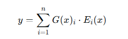 AI Visual Insight: This image shows the mathematical expression for MoE output as a weighted sum of expert outputs using gating weights. It emphasizes the sparse weight vector G(x) produced by the router, which is the core formula behind “large parameter capacity but sparse activation per forward pass.”
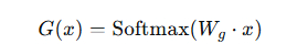 AI Visual Insight: This image shows how the gating network maps input into an expert score distribution, typically via a linear transformation followed by softmax and then Top-k selection. It makes clear that the router itself is a lightweight module rather than the main compute-heavy component.
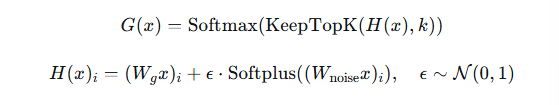 AI Visual Insight: This image highlights the strategy of injecting noise into gating scores to increase exploration and mitigate expert collapse and over-concentrated routing. This directly relates to load balancing and training stability.
The core logic of sparse routing can be compressed into three steps
# Minimal pseudo-implementation of MoE Top-k routing

def moe_forward(x, router, experts, k=2):
    scores = router(x)                        # Compute a score for each expert
    topk_idx = scores.argsort()[-k:]          # Select the top-k scoring experts
    output = 0
    for i in topk_idx:
        output += scores[i] * experts[i](x)   # Aggregate outputs from activated experts only
    return output
This code shows that MoE saves computation by “computing only a small subset of experts,” not by reducing the total number of model parameters.
MoE delivers value in both training and inference
| Dimension | Dense FFN | MoE |
|---|---|---|
| Parameter Scale | Grows linearly with layer width | Can scale much further |
| Active Parameters per Forward Pass | All participate | Only Top-k experts |
| Training Difficulty | Standard stability issues | Routing and load balancing |
| Deployment Benefit | Stable and simple | Higher capacity density |
| Representative Models | GPT-style dense models | Switch, Mixtral, DeepSeek-MoE |
When a model needs larger capacity under a limited compute budget, MoE is often more effective than simply scaling width.
The three Transformer architectures target generation, understanding, and sequence transformation respectively
Decoder-Only uses causal masking, so each position can see only previous tokens. That makes it a natural fit for autoregressive generation, which is why GPT, LLaMA, and Qwen all follow this paradigm. It scales well and has become the de facto standard for general-purpose large language models.
Encoder-Only uses bidirectional attention and is better suited to understanding tasks such as classification, named entity recognition, and retrieval encoding. Encoder-Decoder combines bidirectional encoding with autoregressive decoding, making it a more natural fit for seq2seq tasks such as translation, summarization, and rewriting.
You can identify the right architecture quickly from the masking pattern
# Choose a Transformer architecture based on the task

def choose_arch(task_type):
    if task_type in ["chat", "generation", "codegen"]:
        return "Decoder-Only"     # Best for autoregressive generation
    if task_type in ["classification", "ner", "retrieval"]:
        return "Encoder-Only"     # Best for bidirectional understanding
    if task_type in ["translation", "summarization", "rewrite"]:
        return "Encoder-Decoder"  # Best for sequence transformation
    return "Depends"
This code establishes a direct mapping between mainstream Transformer architectures and task categories.
The key to architecture selection is not sophistication, but task fit
| Architecture | Attention Pattern | Strengths | Typical Tasks |
|---|---|---|---|
| Decoder-Only | Causal masking | General-purpose generation, strong scalability | Dialogue, code generation, completion |
| Encoder-Only | Bidirectional visibility | Strong understanding, efficient fine-tuning | Classification, retrieval, sequence labeling |
| Encoder-Decoder | Encoding + decoding | Strong sequence transformation | Translation, summarization, rewriting |
If your goal is to unify multiple tasks and maximize generation capability, choose Decoder-Only. If you want high-quality semantic encoding, choose Encoder-Only. If the input and output structures differ significantly, prefer Encoder-Decoder.
The main line of the modern large-model technology stack is now very clear
At the embedding layer, dynamic contextual representations have replaced static lookup tables. At the attention layer, GQA is becoming the inference standard. For capacity scaling, MoE makes hundred-billion-parameter systems more practical. At the system level, Decoder-Only dominates general-purpose generation, while the other two architectures still retain strong advantages in specialized tasks.
Understanding these four trends matters more than memorizing model names in isolation, because together they define the design boundaries of modern Transformers: expressive power, deployment efficiency, scalable capacity, and task fit.
FAQ
1. Why haven’t Word2Vec and GloVe become completely obsolete today?
Because they are cheap to train, extremely fast at inference, and simple to implement. They still work well in cost-sensitive scenarios such as lightweight retrieval, clustering, and recommendation. When you do not need deep contextual understanding, static vectors still have practical engineering value.
2. Why do mainstream large models prefer GQA instead of continuing to use standard MHA?
The core reason is that KV cache cost becomes too high during long-sequence inference. GQA offers a better balance among memory usage, bandwidth pressure, and model quality, making it better suited to production-grade deployment.
3. Does MoE always make inference faster?
Not necessarily. MoE’s advantage is that it preserves controllable compute at larger capacity, but routing, cross-device communication, and uneven expert utilization can all introduce extra overhead. With good design, it improves capacity efficiency, but that does not mean it is universally faster in every scenario.
Core Summary: This article systematically outlines four major trends in the modern Transformer stack: embeddings evolving from Word2Vec and GloVe to dynamic contextual representations, attention shifting from MHA toward GQA and MQA, MoE expanding capacity through sparse activation, and the application differences and selection logic among Decoder-Only, Encoder-Only, and Encoder-Decoder architectures.