2026 Huazhong Cup Problem A Reengineered: Urban Green Logistics Scheduling with ALNS and Rolling Horizon Optimization

This article focuses on 2026 Huazhong Cup Problem A, the Urban Green Logistics Delivery Scheduling Model. Its core idea is to use Adaptive Large Neighborhood Search (ALNS), time-dependent road network modeling, and rolling horizon rescheduling to solve a complex VRPTW variant that combines a heterogeneous fleet, soft time windows, energy consumption costs, and green traffic restrictions. Keywords: ALNS, green logistics, dynamic scheduling.

Technical specifications show the problem scale and modeling focus

Parameter	Details
Problem Type	HF-TDVRPTW / Dynamic VRPTW
Primary Language	Python
Modeling Scope	98 customer locations, 2,169 orders, heterogeneous mixed fleet
Core Constraints	Weight, volume, soft time windows, time-dependent speed, green-zone restrictions
Solution Strategy	ALNS + Split Delivery + Rolling Horizon
License / Copyright	CC 4.0 BY-SA (stated in the source attribution)
Star Count	Not provided in the original data
Core Dependencies	NumPy, heuristic insertion, penalty functions, space-time network

This competition problem is essentially a highly coupled green logistics optimization problem

The problem requires coordinated scheduling of fuel vehicles and new energy vehicles in a single-day delivery scenario. The challenge is not simply to find the shortest path for each route. The real difficulty lies in the multi-objective coupling among cost, legal feasibility, service timeliness, and carbon emissions.

The original problem can be abstracted as a Heterogeneous Fleet Vehicle Routing Problem with Time Windows (HFVRPTW), further augmented by a time-dependent traffic network and dynamic event response. That makes it much closer to an industrial-grade instant delivery scheduling system than a standard CVRP or a traditional VRPTW.

AI Visual Insight: The image serves as a cover-style visual introduction to the competition topic, emphasizing urban green logistics delivery scheduling. It is a thematic promotional graphic rather than an algorithmic diagram, mainly conveying the problem context and competition background.

Exact solvers cannot brute-force this problem efficiently

When the number of nodes approaches 100, the order count exceeds 2,000, and each route cost depends on departure time, vehicle type, and load factor, the model grows very quickly. If you directly build a large-scale MILP at that point, both the variable dimension and the number of constraints become difficult to control.

A more effective approach is to first model physical cost evaluation accurately, then use heuristic search to iterate quickly inside the feasible space. That is exactly why ALNS outperforms a purely exact approach for this problem.

Static optimization must first resolve the time-dependent network and energy cost model

The core of Problem 1 is to find the minimum total cost routes without green-zone traffic restrictions. Here, “total cost” is not a single distance-based metric. It is a combination of travel time, fuel or electricity consumption, load-factor penalties, and service time-window penalty functions.

Time-dependent traffic means the travel time over the same road segment changes by departure time. As a result, edge cost is no longer a constant. Instead, it becomes a function of the departure time. In practice, this is usually modeled with piecewise speed tables or discrete integral approximations.

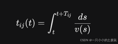AI Visual Insight: The image presents a mathematical expression for travel time under a time-dependent road network. Its core meaning is to split a fixed travel distance across multiple traffic-speed intervals and integrate or accumulate the segment costs to derive the true travel time as a function of departure time.

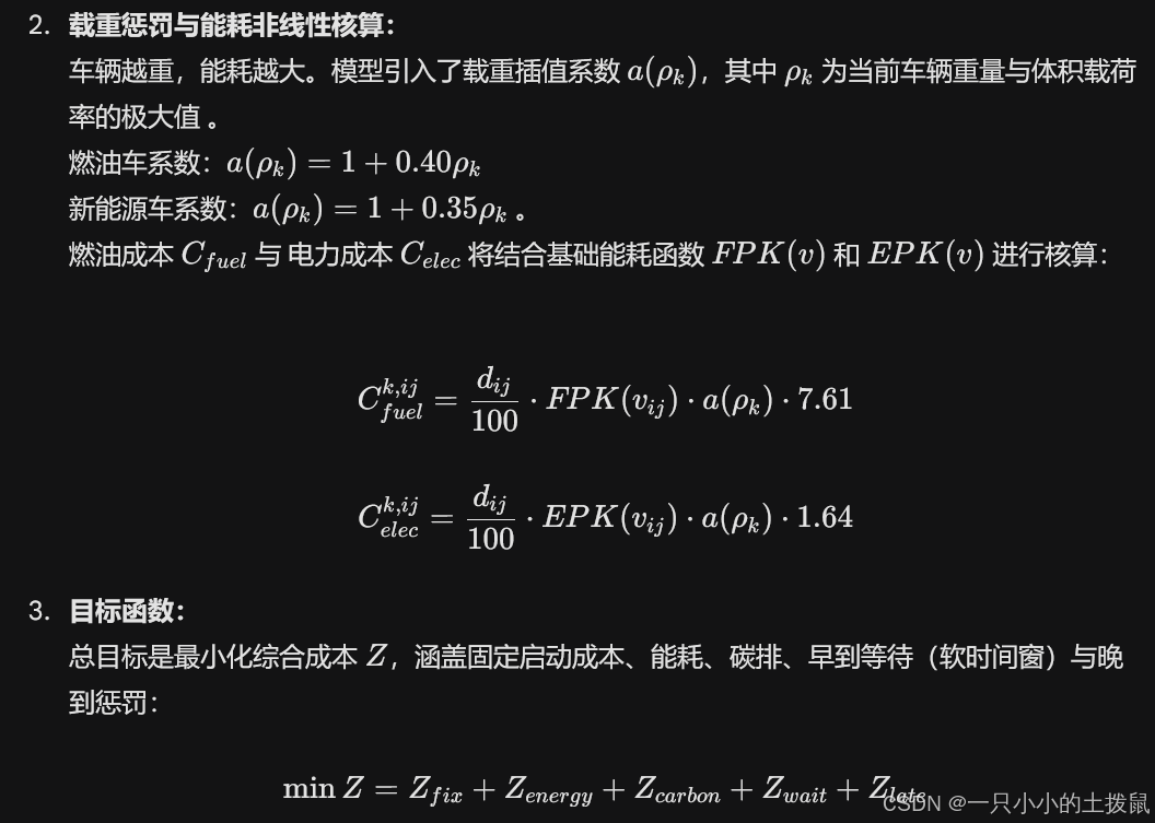AI Visual Insight: The image further illustrates the piecewise calculation structure of travel time or cost, emphasizing the dynamic relationship among feasible distance, accumulated duration, and traffic-state transitions such as peak, off-peak, and free-flow periods.

Time-dependent speed and energy use can be unified in a single simulation function

import numpy as np

def calculate_travel_time_and_cost(dist, start_time, vehicle_type, load_rate):
    """Calculate travel time and energy cost under time-dependent speed."""
    speed_map = {0: 9.8, 1: 35.4, 2: 55.3}  # Vehicle speeds under different traffic states
    current_time = start_time
    remaining_dist = dist
    total_energy_cost = 0.0

    while remaining_dist > 0:
        traffic_state = get_traffic_state(current_time)  # Determine the current congestion state
        v = speed_map[traffic_state]
        time_to_next_state = get_time_to_next_state(current_time)  # Time remaining until the next interval
        dist_in_state = v * time_to_next_state
        step_dist = min(remaining_dist, dist_in_state)
        step_time = step_dist / v

        if vehicle_type == "Fuel":
            a_rho = 1 + 0.40 * load_rate  # Load-factor penalty for fuel vehicles
            fpk = 0.0025 * (v ** 2) - 0.2554 * v + 31.75
            total_energy_cost += (step_dist / 100) * fpk * a_rho * 7.61
        else:
            a_rho = 1 + 0.35 * load_rate  # Load-factor penalty for electric vehicles
            epk = 0.0014 * (v ** 2) - 0.12 * v + 36.19
            total_energy_cost += (step_dist / 100) * epk * a_rho * 1.64

        remaining_dist -= step_dist
        current_time += step_time  # Advance the physical time axis

    return current_time - start_time, total_energy_cost

This function completes a unified evaluation of time-dependent speed, vehicle-specific energy consumption, and load-factor penalties. It is the most critical cost evaluation kernel in the static optimization stage.

ALNS is well suited for near-optimal search in a large feasible region

Because the demand of a single customer may exceed the capacity of one vehicle, the original approach introduces Split Delivery. This strategy matters because it transforms “infeasible to serve” into “service can be split,” which significantly expands the feasible region.

The value of ALNS lies in the fact that it does not rely on a fixed neighborhood. Instead, it performs adaptive search through combinations of destroy and repair operators. Common destroy operators include worst removal, random removal, and related removal. Common repair operators include greedy insertion and regret-based insertion.

A practical solution framework should include four modules

1. Initial solution construction: quickly build a feasible solution based on time-window urgency and regional clustering.
2. Destroy phase: remove part of the customers to break local optima.
3. Repair phase: reinsert orders using minimum incremental cost or regret value.
4. Weight update: dynamically adjust selection probabilities based on historical operator performance.

def alns_iteration(solution, destroy_ops, repair_ops, scores, temperature):
    destroy = select_operator(destroy_ops, scores["destroy"])  # Select a destroy operator by weight
    repair = select_operator(repair_ops, scores["repair"])    # Select a repair operator by weight

    partial = destroy(solution)                                # Disrupt the current solution
    candidate = repair(partial)                                # Rebuild a candidate solution

    if accept(candidate, solution, temperature):               # Simulated annealing acceptance criterion
        solution = candidate
        update_scores(scores, destroy, repair, reward=1)

    return solution

This code skeleton shows the core ALNS loop: operator selection, solution destruction, solution repair, acceptance, and adaptive learning.

Green-zone restrictions transform a standard routing problem into a space-time blocking problem

Problem 2 introduces a green delivery zone restriction from 8:00 to 16:00: fuel vehicles are not allowed to enter the central area during that time window. At this point, the constraint is no longer just “can the vehicle reach the customer.” It becomes “can the vehicle legally reach the customer at that specific time.”

This type of constraint is essentially a space-time reachability cut. If a customer is located inside the green zone and the upper bound of its time window is earlier than 16:00, then service by a fuel vehicle should be marked directly infeasible in the model.

AI Visual Insight: The image shows the mathematical formulation of the green-zone restriction. The key technical idea is to jointly restrict service feasibility using the customer’s area label, the vehicle type set, and the arrival time. In essence, this is a time-dependent reachability constraint with regional blocking.

A more robust implementation uses a two-layer design: rule-first assignment plus search penalties

During initialization, prioritize assigning customers in the green zone with tight time windows to new energy vehicles so that baseline feasibility is satisfied early. After entering ALNS, use large penalties to block illegal insertions and prevent the search from repeatedly violating hard constraints.

This design is more stable than post hoc repair because it prunes some infeasible combinations before the search starts and reduces wasted iterations.

Dynamic disruptions require rolling horizon rescheduling capability

Problem 3 is the closest to a real business scenario: order cancellations, urgent new orders, address changes, and time-window adjustments can all invalidate the original routes. If you recompute the entire plan globally whenever an event occurs, the cost is too high and the already executed plan becomes unstable.

That is why rolling horizon should be used. At the event time, freeze all completed and non-interruptible segments, and only re-optimize the remaining decision space. This approach responds quickly while controlling the degree of disruption to the original plan.

AI Visual Insight: The image presents the joint objective function for dynamic rescheduling. In addition to the remaining transportation cost, it explicitly includes a disruption penalty for deviation from the original plan, reflecting a dual-objective balance between operational efficiency and plan stability.

Regret-based insertion is a better fit for dynamic order insertion

def dynamic_rescheduling(event_time, new_orders, canceled_orders, current_routes, vehicle_status):
    """Dynamic rescheduling under a rolling horizon."""
    for route in current_routes:
        route.customers = [c for c in route.customers if c not in canceled_orders]  # Remove canceled orders first

    for vehicle in vehicle_status:
        vehicle.update_state_at_time(event_time)  # Freeze vehicle states at the event time

    unassigned_orders = new_orders.copy()
    while unassigned_orders:
        best_order, best_plan, max_regret = None, None, -float("inf")

        for order in unassigned_orders:
            insertions = find_all_feasible_insertions(order, current_routes, vehicle_status)

            if len(insertions) >= 2:
                regret = insertions[1]["cost"] - insertions[0]["cost"]  # Compute the regret value
            elif len(insertions) == 1:
                regret = float("inf")
            else:
                insertions = [{"vehicle": allocate_new_vehicle(), "cost": calculate_new_dispatch_cost(order)}]
                regret = float("inf")

            if regret > max_regret:
                best_order, best_plan, max_regret = order, insertions[0], regret

        execute_insertion(best_order, best_plan, current_routes)  # Execute the most urgent insertion
        unassigned_orders.remove(best_order)

    return current_routes

This code captures the core idea of dynamic scheduling: prioritize orders that will become much more expensive if you do not insert them now, thereby improving the robustness of local replanning.

The engineering value of this solution comes from decomposing complex constraints into computable modules

The most reusable lesson from this problem is not any single algorithm name. It is the layered modeling approach: realistic cost simulation at the bottom layer, heuristic search in the middle layer, and dynamic event replanning at the top layer.

From an engineering perspective, the same method also applies to instant retail, urban cold-chain distribution, and front-warehouse delivery for community group buying. As long as the scenario includes a mixed fleet, time windows, regional policy constraints, and dynamic orders, this framework has direct transfer value.

FAQ

Q1: Why choose ALNS first instead of a genetic algorithm or pure MILP?

ALNS adapts more naturally to complex constraints and can explore a large solution space quickly through multiple destroy and repair operators. Compared with pure MILP, it scales better. Compared with a generic genetic algorithm, it is easier to embed time windows, traffic restrictions, and dynamic insertion rules.

Q2: What is the most common modeling mistake in green-zone restriction constraints?

The most common mistake is to restrict only whether the customer is inside the green zone without including the arrival time in the feasibility condition. The correct approach is to jointly consider region, vehicle type, and arrival time.

Q3: Why not recompute the whole schedule globally every time dynamic rescheduling is triggered?

Because global recomputation disrupts the already executed plan and becomes too expensive when events occur frequently. Rolling horizon freezes the executed portion and only optimizes the remaining routes, which provides a better balance between responsiveness and stability.

[AI Readability Summary]

This article reconstructs the original material of 2026 Huazhong Cup Problem A and distills a three-layer solution framework for urban green logistics delivery: static mixed-fleet route optimization, space-time constraint reconstruction under green-zone restrictions, and rolling horizon rescheduling under dynamic disruptions. It also provides a practical ALNS modeling strategy and implementation-ready code skeletons.