PEFT Explained: Efficient Fine-Tuning for LLMs from Prompt Tuning to LoRA - Devuly | Smart Analytics for Developers & Projects

For production LLM applications, PEFT adapts models to downstream tasks at low cost by freezing most pretrained parameters and training only a small set of incremental parameters. It solves the high memory usage, slow training, and heavy deployment footprint of full fine-tuning. Keywords: PEFT, LoRA, Prompt Tuning.

Table of Contents

Technical specifications at a glance

Parameter	Details
Technical focus	Parameter-efficient fine-tuning for large language models
Primary language	Python
Mainstream frameworks	Hugging Face Transformers, PEFT
Applicable models	Transformer models such as BERT, T5, LLaMA, and Qwen
Typical protocols/paradigms	Supervised fine-tuning, instruction tuning, decoding-time calibration
Representative methods	Prompt Tuning, Prefix Tuning, Adapter, BitFit, Child-Tuning, LoRA
Typical hardware gains	For a 7B model, memory usage can drop from about 60 GB for full fine-tuning to about 23 GB with LoRA
Core dependencies	torch, transformers, peft, accelerate
GitHub stars	Not provided in the source input; refer to the live Hugging Face PEFT repository data

PEFT has become the default engineering path for production LLMs

The bottleneck of full fine-tuning is not whether you can train a model once, but whether you can keep training it sustainably. Once model size reaches 7B, 13B, or even 70B parameters, GPU memory requirements, training time, and storage for model replicas all scale up rapidly.

The core idea behind PEFT is straightforward: freeze the base model and compute gradients only for a small number of newly added parameters or a selected subset of existing parameters. This preserves pretrained knowledge while keeping task adaptation costs within a manageable range.

Prompt engineering and full fine-tuning are both limited in practice

Prompt engineering works well for zero-shot or few-shot exploration, but its performance depends heavily on prompt design, and inference cost increases with context length. It is better suited for rapid validation than as a stable production strategy.

Full fine-tuning sits at the other extreme. It can deliver strong results, but it is highly sensitive to training memory and optimizer state size. For a 7B model, a full training pipeline is often beyond what consumer GPUs can handle.

from peft import LoraConfig, get_peft_model
from transformers import AutoModelForCausalLM

model = AutoModelForCausalLM.from_pretrained("Qwen/Qwen2-7B-Instruct")

config = LoraConfig(
    r=8,                 # Low-rank dimension, which determines the number of trainable parameters
    lora_alpha=16,       # Scaling factor that controls the strength of incremental updates
    lora_dropout=0.05,   # Regularization to reduce overfitting risk on small datasets
    target_modules=["q_proj", "v_proj"]  # Inject only into key attention projection layers
)

model = get_peft_model(model, config)
model.print_trainable_parameters()  # Print the ratio of trainable parameters

This code shows how to inject LoRA into a base model and train only a small set of incremental parameters.

PEFT can be divided into three main technical routes

The first category is parameter addition, which adds small modules at the input, hidden-layer, or output side. The second is parameter selection, which updates only a subset of the original model parameters. The third is low-rank adaptation, which approximates weight updates with low-rank factorization.

The essential difference between these routes is where the parameters are modified and how the update space is constrained.

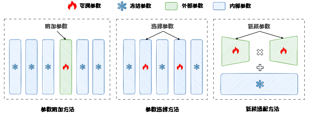AI Visual Insight: This diagram compares the three PEFT routes—parameter addition, parameter selection, and low-rank adaptation—from a structural perspective. It highlights the design principle of freezing backbone parameters while training only localized modules, making it useful for understanding differences in parameter injection points and gradient flow.

Input-side methods are best represented by Prompt Tuning

Prompt Tuning prepends a set of trainable soft prompt vectors before the input embeddings. During training, only these continuous vectors are updated, while the original model weights remain untouched. This keeps the parameter count extremely small and makes the approach especially suitable for multi-task sharing on a single base model.

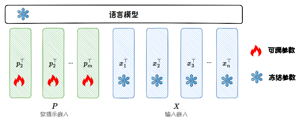AI Visual Insight: The figure shows how soft prompt vectors are concatenated with the original token embeddings. It emphasizes that the trainable prompt enters the Transformer encoder as continuous parameters rather than discrete text prompts, clearly illustrating Prompt Tuning as an input-level parameter injection mechanism.

Internal model methods focus on adaptation inside intermediate layers

Prefix Tuning does more than modify the input. It injects trainable prefixes into the Key/Value paths of attention layers, so it usually has stronger expressive power than Prompt Tuning, although it also introduces more trainable parameters.

Adapters insert a bottleneck module after each attention or feed-forward layer. They first project down, then apply a nonlinear transformation, and finally project back up, allowing the model to learn task-specific features at very low cost.

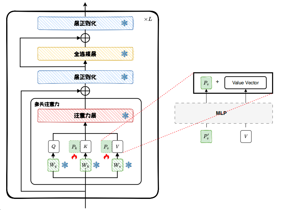AI Visual Insight: This diagram illustrates how Prefix Tuning inserts prefix vectors into the attention modules of multiple Transformer layers. It highlights that the prefix affects not only the input representation but also the attention key-value cache directly, which is a major reason it is more expressive than input-level soft prompts.

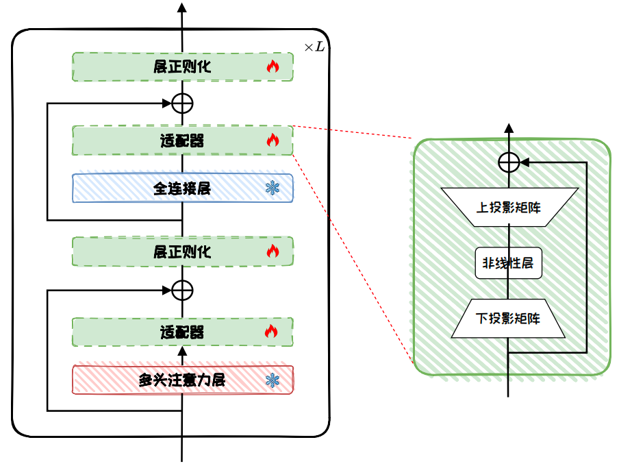AI Visual Insight: The left side of the figure shows Adapters inserted after multi-head attention and feed-forward layers, while the right side breaks down the bottleneck structure into down-projection, activation, and up-projection. This clearly shows how Adapters rewrite local representations with small modules instead of modifying entire layer weights.

from peft import PrefixTuningConfig, TaskType

prefix_config = PrefixTuningConfig(
    task_type=TaskType.CAUSAL_LM,
    num_virtual_tokens=20,      # Prefix length; longer prefixes provide stronger expressiveness
    encoder_hidden_size=768     # Hidden size of the prefix encoding MLP
)

This configuration snippet highlights the two key hyperparameters in Prefix Tuning: prefix length and encoder dimension.

Output-side methods fit black-box models and extremely large models

Proxy-Tuning does not directly access the weights of the large model. Instead, it combines the logits of a proxy model, an expert model, and an anti-expert model during decoding. This makes it especially suitable for API-based models with inaccessible weights, or for extremely large models that cannot be trained directly.

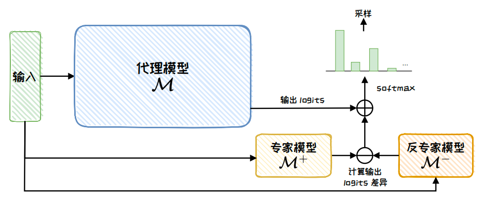AI Visual Insight: The figure shows the logits fusion workflow among the proxy model, expert model, and anti-expert model during decoding. It highlights that the method customizes behavior without changing the main model weights, relying instead on output distribution reweighting.

Parameter selection methods trade smaller updates for lower overhead

BitFit takes the most aggressive approach: it trains only bias terms and the task head. Because bias parameters account for only a tiny fraction of total parameters, training is stable and inexpensive, although its performance ceiling depends on model scale and task difficulty.

Child-Tuning goes one step further by using a mask matrix to restrict gradients to a subnetwork. This can be done through random sampling or by using Fisher information to select more important parameter subsets.

import torch

# grad_mask indicates which parameter positions can be updated in the current iteration
param.grad = param.grad * grad_mask  # Keep only subnetwork gradients and zero out the rest
optimizer.step()

This code summarizes the core idea of Child-Tuning: selective updates through gradient masking.

LoRA became the mainstream choice because it balances quality and engineering practicality

LoRA assumes that the weight update matrix itself is low-rank, so it factorizes the incremental matrix into two small matrices, A and B, and trains only them. The original weights stay frozen, and the training scale drops from d×k to r×(d+k).

This brings three direct benefits: lower memory usage, faster training, and the ability to merge the update back into the original weights at inference time with almost no additional latency. That is why LoRA has become the most widely used PEFT method in the open-source ecosystem.

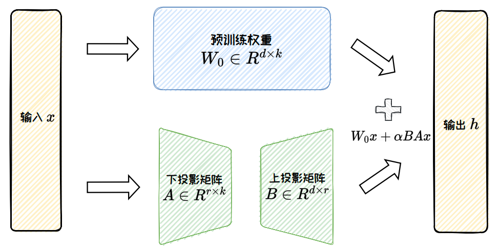AI Visual Insight: The figure decomposes a large weight update matrix into the product of two low-rank matrices. It visually explains how LoRA approximates full weight updates with a small number of parameters while keeping the backbone model frozen during training.

The key conclusion about LoRA is that low rank does not mean low capability

Consider an FFN layer in LLaMA2-7B. Full fine-tuning may require updating about 45 million parameters, while LoRA with r=4 needs only about 60,000 trainable parameters—less than one-thousandth of the original scale.

LoRA does have a low-rank bottleneck, which is why variants such as AdaLoRA, ReLoRA, and DoRA have emerged. They improve performance and stability through dynamic rank allocation, periodic merge-and-reset cycles, and decoupling direction from magnitude, respectively.

PEFT engineering practices have matured into a standard toolchain

The most mature implementation today is Hugging Face PEFT. It integrates well with Transformers, Accelerate, quantization tools, and distributed training components, making it suitable for the full path from experimentation to production.

For method selection, you can follow a simple rule of thumb: if GPU memory is extremely limited, choose Prompt Tuning or BitFit; if you need stronger and more stable generalization, choose Adapters or Prefix Tuning; if you want the best balance between quality and deployment efficiency, start with LoRA and its variants.

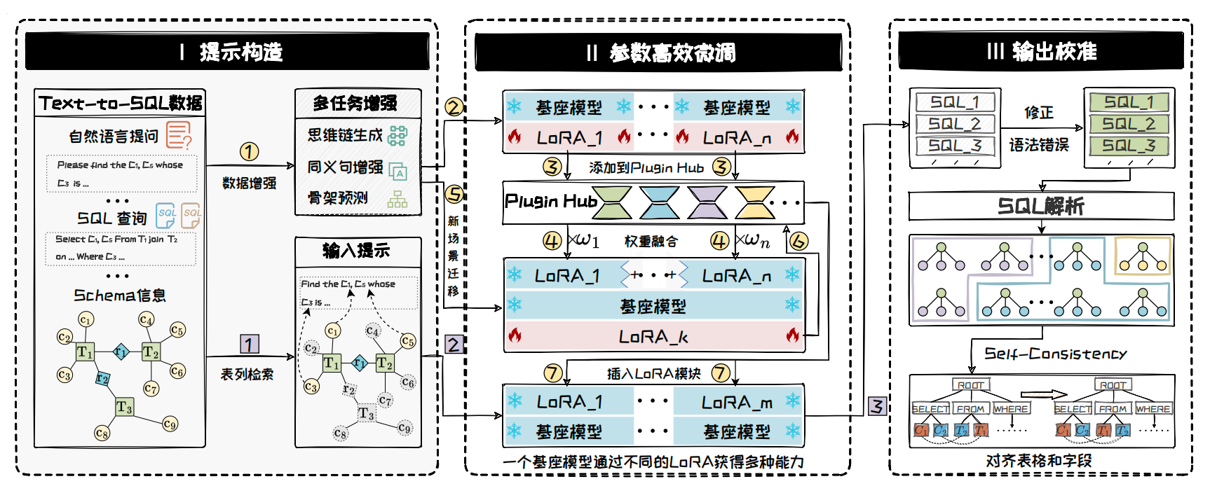AI Visual Insight: This figure shows a complete workflow for a financial Text-to-SQL scenario, including prompt construction, PEFT fine-tuning, LoRA composition, and output calibration. It illustrates how PEFT has evolved from a standalone training trick into a production-ready industry workflow.

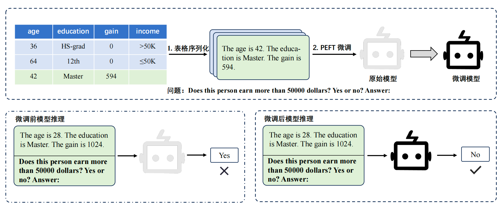AI Visual Insight: The figure shows how TabLLM serializes tabular samples into natural language and uses LoRA for few-shot adaptation. It highlights the data re-representation strategy used to connect tabular tasks with language models.

FAQ

Q1: When should you choose LoRA over full fine-tuning?

A1: Choose LoRA when the model size exceeds the memory limit of a single GPU, task data is limited, and you need to iterate quickly across multiple task versions. It offers the best balance among quality, memory efficiency, and deployment complexity.

Q2: What is the essential difference between Prompt Tuning and Prefix Tuning?

A2: Prompt Tuning adds soft prompts only before the input embeddings. Prefix Tuning further injects trainable prefixes into the Key/Value paths of attention modules across layers, which gives it stronger expressive power at the cost of more trainable parameters.

Q3: Is PEFT only useful for text generation tasks?

A3: No. PEFT is already widely used in classification, retrieval, question answering, Text-to-SQL, tabular analysis, vision-language models, and diffusion models. As long as the base model is large and the task requires low-cost adaptation, PEFT is valuable.

Core summary: This article systematically explains the core logic of Parameter-Efficient Fine-Tuning (PEFT), covering the principles, cost advantages, and engineering practices of Prompt Tuning, Prefix Tuning, Adapter, BitFit, Child-Tuning, and LoRA, helping developers adapt large models under limited GPU memory constraints.