Advanced MySQL Single-Table Queries: UPDATE, DELETE, Aggregate Functions, and GROUP BY in Practice - Devuly | Smart Analytics for Developers & Projects

This article focuses on advanced MySQL single-table querying. It systematically explains updates, deletes, aggregate statistics, and grouped queries, addressing common pain points such as accidental SQL mass updates or deletes, inconsistent counting logic, and confusion between HAVING and WHERE. Keywords: MySQL, GROUP BY, aggregate functions.

Table of Contents

Technical Specification Snapshot

Parameter	Details
Primary Language	SQL / MySQL
Supported Environments	MySQL 5.7+ / 8.x
Operation Types	`UPDATE`, `DELETE`, `INSERT SELECT`, `GROUP BY`
Article Focus	Practical data modification and statistical analysis
Star Count	Not provided in the source material
Core Dependencies	MySQL Server, command-line client, or GUI client

This article organizes the most common data modification and statistical capabilities in MySQL

In the second half of single-table querying, what truly determines development efficiency is not SELECT *, but updates, deletes, aggregation, and grouping. These operations directly affect data correctness, reporting consistency, and production safety.

The core focus of the original material is clear: it centers on UPDATE, DELETE, TRUNCATE, aggregate functions, and GROUP BY, making it ideal for developers who want to quickly strengthen their practical database skills after learning the basics.

UPDATE essentially modifies the result set returned by a query

UPDATE does not blindly modify an entire table. It first identifies a result set, then updates the matched rows. That is why WHERE, ORDER BY, and LIMIT often appear together.

UPDATE exam_result
SET math = 80
WHERE name = '孙悟空'; -- Only update the specified student's math score

This SQL statement performs a precise single-row update and avoids affecting unrelated data.

If you need to update multiple fields at the same time, you can assign values consecutively in SET. In production environments, this pattern commonly appears in status synchronization and batch corrections.

UPDATE exam_result
SET math = 60,        -- Update the math score
    chinese = 70      -- Update the Chinese score at the same time
WHERE name = '曹孟德'; -- Target the intended row

This SQL statement demonstrates the standard way to update multiple columns in a single statement.

Updating based on existing values is a common pattern and closer to real business scenarios

Many people mistakenly write math += 30, but MySQL does not support that syntax. You must explicitly write math = math + 30.

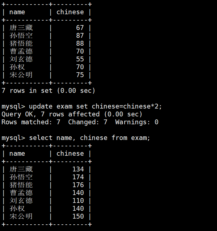
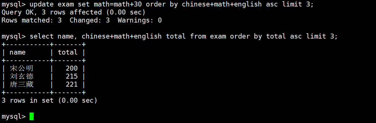
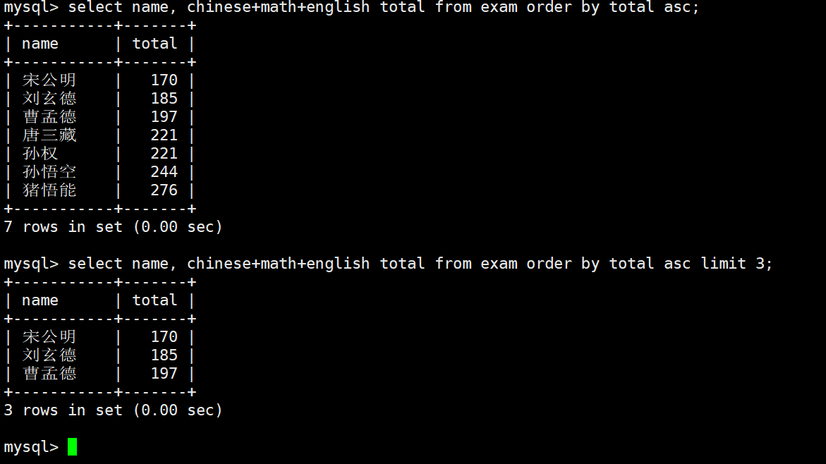
UPDATE exam_result
SET math = math + 30              -- Add 30 to the original score
ORDER BY chinese + math + english -- Sort by total score in ascending order
LIMIT 3;                          -- Only update the bottom three students

This SQL statement shows the typical technique of partially updating rows based on sorted results.

An update without WHERE is dangerous because it affects the entire table. Unless you are performing intentional data initialization, you should first run a SELECT with the same condition to verify the affected scope.

UPDATE exam_result
SET chinese = chinese * 2; -- No WHERE clause, so the entire table will be updated

This SQL statement is a reminder that full-table updates are syntactically valid but operationally high-risk.

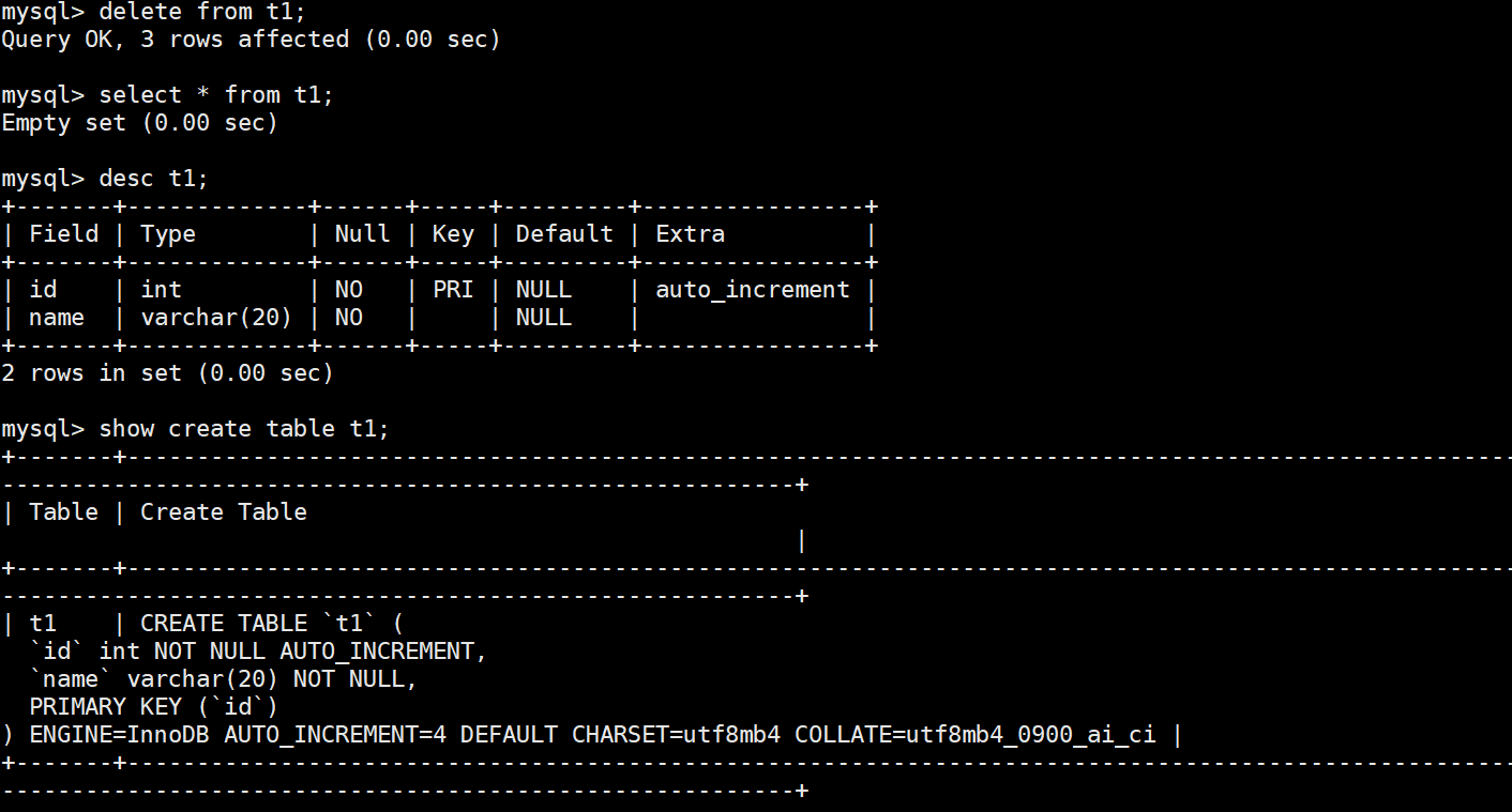
The key to delete statements is not writing them, but understanding the cost differences

DELETE and TRUNCATE may both clear data, but their underlying behavior and usage scenarios are completely different. One is more transaction-oriented, while the other is more suitable for fast resets.

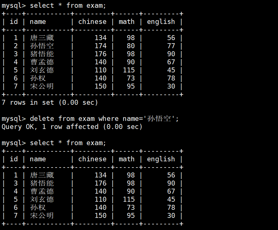
DELETE FROM exam_result
WHERE name = '孙悟空'; -- Delete the specified row

This SQL statement is suitable for deleting a subset of data by condition.

DELETE FROM table_name; -- Delete all rows, but usually does not reset the auto-increment value

This SQL statement removes data row by row and is suitable when you need transactional semantics or possible condition-based extensions.

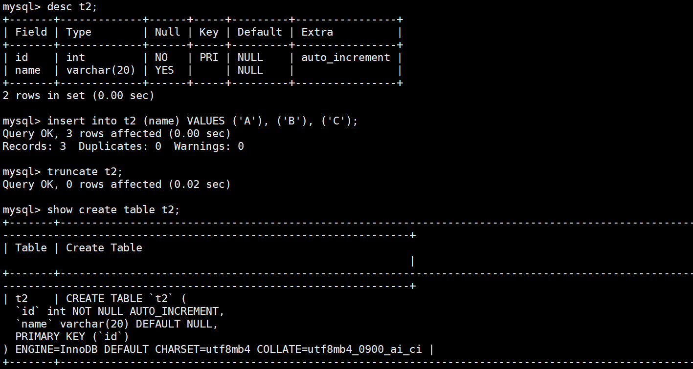
TRUNCATE behaves more like rebuilding a table than deleting rows one by one

TRUNCATE is fast, but the tradeoff is reduced control granularity. It usually resets the auto-increment value and cannot delete only part of the data the way a normal DELETE can.

TRUNCATE table_name; -- Quickly clear the table and usually reset the auto-increment primary key

This SQL statement is useful in test environments when you need to recycle table data quickly.

You can remember the differences directly: DELETE supports conditional deletion, can be rolled back, and is relatively slower; TRUNCATE clears data faster, usually resets auto-increment, and provides weaker transaction-level control.

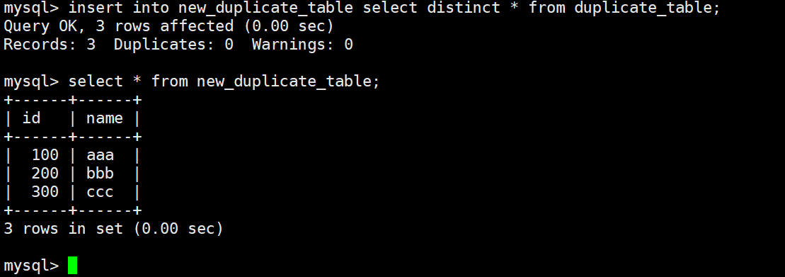
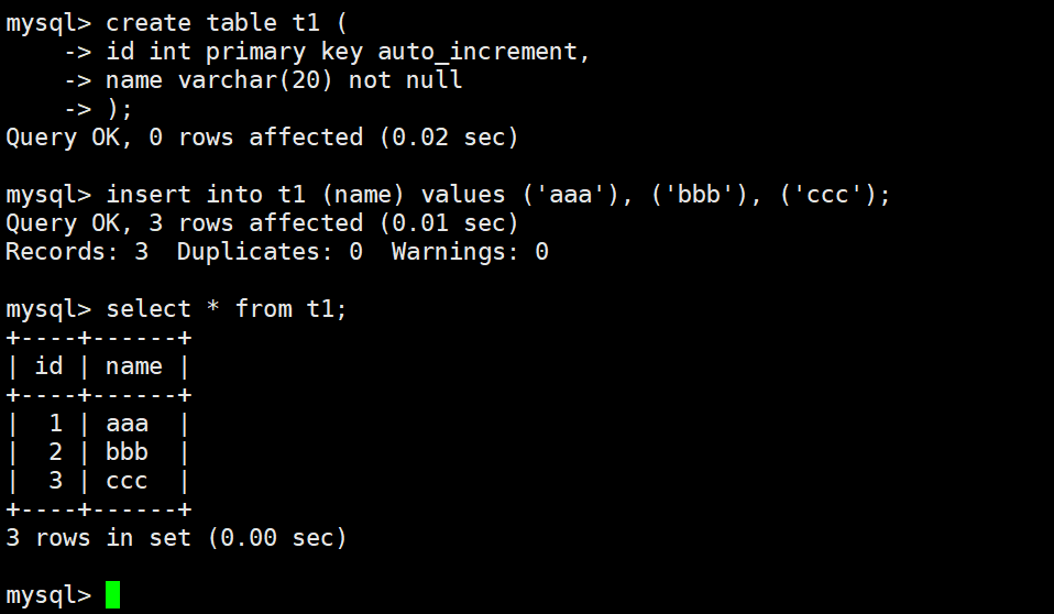
Inserting query results is a practical pattern for deduplication and migration

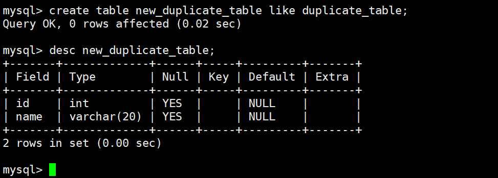
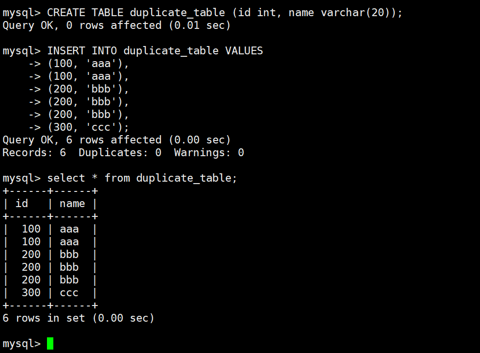
When an old table contains duplicate data, the safest approach is not to force-delete duplicates in place. Instead, create a new table with the same structure and write clean data into it through SELECT DISTINCT.

CREATE TABLE new_table LIKE old_table; -- Copy the table structure

INSERT INTO new_table
SELECT DISTINCT * FROM old_table;      -- Insert deduplicated data into the new table

This pair of SQL statements performs low-risk data deduplication.

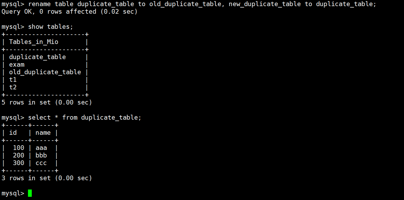
If you also want a near-transparent business switchover, you can complete an atomic replacement by renaming tables. This approach is commonly used in historical dirty data remediation.

RENAME TABLE old_table TO backup_table, -- Back up the old table first
             new_table TO old_table;    -- Replace it with the new table

This SQL statement completes a table-level switchover in a very short time.

Aggregate functions determine whether statistical queries are accurate

Aggregate functions primarily answer questions like “how many,” “what is the total,” “what is the average,” and “what are the maximum and minimum.” The most common ones are COUNT, SUM, AVG, MAX, and MIN.

SELECT COUNT(*) FROM students;               -- Count the total number of rows
SELECT COUNT(qq) FROM students;             -- Count only rows where qq is not NULL
SELECT COUNT(DISTINCT math) FROM exam_result; -- Count distinct math scores

These SQL statements explain the difference in counting logic among COUNT(*), COUNT(column), and COUNT(DISTINCT column).

Sums, averages, and extreme values are commonly used in reports, leaderboards, and threshold checks. Note that expressions can also participate directly in aggregation.

SELECT SUM(math) FROM exam_result;                          -- Total math score
SELECT AVG(chinese + math + english) FROM exam_result;     -- Average total score
SELECT MAX(english) FROM exam_result;                       -- Highest English score
SELECT MIN(math) FROM exam_result WHERE math > 70;         -- Lowest math score among scores greater than 70

These SQL statements show the most common patterns in statistical analysis.

GROUP BY compresses detailed rows into analyzable grouped results

The value of GROUP BY lies in aggregating multiple rows by dimension, such as department, role, class, or date. It is typically used together with aggregate functions.

SELECT deptno, AVG(sal), MAX(sal)
FROM EMP
GROUP BY deptno; -- Group by department, then calculate average and maximum salary

This SQL statement outputs one summary row per department.

Grouping by multiple fields is also common because it gives you finer statistical dimensions. For example, you can group first by department and then by role to observe salary differences.

SELECT deptno, job, AVG(sal)
FROM EMP
GROUP BY deptno, job; -- Group by both department and role

This SQL statement is suitable for building more granular analytical reports.

HAVING filters after grouping, while WHERE filters before grouping

This is a frequent interview topic and one of the easiest concepts for beginners to confuse. WHERE filters raw rows first, while HAVING filters grouped results after aggregation.

SELECT deptno, AVG(sal) AS avg_sal
FROM EMP
GROUP BY deptno
HAVING avg_sal < 2000; -- Keep only departments with an average salary below 2000

This SQL statement continues filtering after grouping has completed.

It is also worth memorizing the common SQL execution order directly: FROM -> WHERE -> GROUP BY -> HAVING -> SELECT -> ORDER BY -> LIMIT. Once you understand this order, many syntax constraints become intuitive.

The original screenshots show the full operation flow and result interfaces

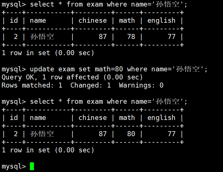
AI Visual Insight: This screenshot most likely shows the execution result of an update statement in a MySQL client. The focus is usually on the number of affected rows, the success message, and changes before and after the update, helping verify whether UPDATE ... WHERE ... matched the intended rows.

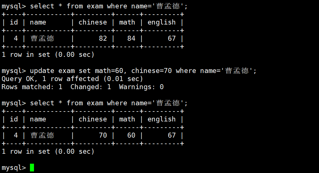
AI Visual Insight: This screenshot likely corresponds to a multi-column update scenario. It may show multiple score columns in the same row being modified at once, emphasizing the batch assignment effect of SET col1 = value1, col2 = value2.

AI Visual Insight: This image may reflect the result of an update based on existing values, such as math = math + 30. The technical focus is expression-based updates rather than static overwrites, which makes it useful for illustrating incremental change logic.

AI Visual Insight: This screenshot may show the result of an update combined with ORDER BY and LIMIT, demonstrating that MySQL can modify a subset of rows after sorting. This pattern is useful for low-score adjustment, bulk correction, and similar scenarios.

AI Visual Insight: This image is likely related to a full-table update or another risky modification. It typically shows a uniform change across many rows and serves as a warning that every record will be affected when WHERE is missing.

AI Visual Insight: This screenshot may correspond to the query result after deleting a single row with DELETE, showing that the data for the specified name has disappeared and emphasizing the precise effect of conditional deletion on the result set.

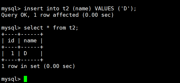
AI Visual Insight: This image may show the empty-table state after a full-table DELETE or TRUNCATE. Typical details include Empty set or a record count of 0, proving that the table data has been cleared.

AI Visual Insight: This screenshot most likely shows the original table data before deduplication, where duplicate rows are visible side by side. Its purpose is to establish a comparison baseline for the SELECT DISTINCT deduplication approach.

AI Visual Insight: This image may show the result after creating the new table or inserting deduplicated data. The key point is that duplicate rows have been collapsed, proving the effectiveness of INSERT INTO ... SELECT DISTINCT ....

AI Visual Insight: This screenshot should correspond to aggregate function queries and may display the return values of COUNT, SUM, or AVG. It is useful for showing that statistical queries typically return a single-row, single-column result.

AI Visual Insight: This image may show the result interface for MAX, MIN, or conditional aggregation. The technical focus is that aggregate functions can work together with WHERE so that rows are filtered before statistics are calculated.

AI Visual Insight: This screenshot likely corresponds to a basic GROUP BY result set, typically displayed as multiple department-level summary rows, where each row represents a group rather than an original record.

AI Visual Insight: This image may show the result set after grouping by multiple fields. The grouping granularity is finer, which makes it easier to compare aggregate differences across department-role combinations.

AI Visual Insight: This screenshot most likely shows grouped results filtered by HAVING. The key point is that only groups satisfying the aggregate condition are kept, which visually distinguishes it from WHERE, which filters raw rows.

These concepts form the core closed loop of MySQL single-table operations

From updates to deletes, and from deduplication and migration to statistical analysis, these statements cover the most common data-processing needs in day-to-day development. The real key is not just knowing how to write them, but also understanding their impact scope, execution phase, and risk boundaries.

When practicing, prioritize these four rules: add conditions before updating or deleting, clarify your counting logic before aggregating, use HAVING for post-group filtering, and confirm whether you need to preserve auto-increment behavior and transactional capabilities before clearing a table.

FAQ

1. Why is it strongly recommended to write `WHERE` first for `UPDATE` and `DELETE`?

Because these statements affect all matched rows by default. When WHERE is missing, the result can range from modifying the entire table to deleting it completely. A safe practice is to preview the affected scope with a SELECT using the same condition first.

2. What is the difference between `COUNT(*)` and `COUNT(column_name)`?

COUNT(*) returns the total number of rows and does not ignore NULL rows at the row level. COUNT(column_name) counts only rows where that column is not NULL. If you need the count of unique values, use COUNT(DISTINCT column_name).

3. How should I distinguish between `WHERE` and `HAVING`?

WHERE filters original rows before grouping, while HAVING filters aggregated results after grouping. If the condition depends on aggregate results such as AVG, COUNT, or SUM, you should generally use HAVING.

Core summary: This article systematically reconstructs advanced MySQL single-table querying knowledge, covering the core syntax, typical examples, and common interview topics for UPDATE, DELETE, TRUNCATE, aggregate functions, GROUP BY, and HAVING. It helps developers quickly master the essential skills for data modification, deletion, statistical analysis, and grouped filtering.