Deep Learning–Driven 3D Reconstruction Pipeline: From Task Definition to Production Deployment

This article outlines the full path of how deep learning is reshaping 3D reconstruction—from task definition and data governance to the geometric front end, deep fusion, appearance recovery, and deployment optimization. The core goal is to improve robustness, generalization, and production readiness. Keywords: 3D reconstruction, deep learning, NeRF.

Technical specifications are summarized below

Parameter	Description
Domain	3D Reconstruction / Machine Vision / Deep Learning
Primary Languages	Python, C++
Common Protocols / Data Interfaces	Image streams, point clouds, RGB-D, LiDAR, SLAM/SfM data interfaces
Popularity Reference	Original blog note: 76, approximately 110,000 views
Core Dependencies	OpenCV, Open3D, PyTorch, COLMAP, NeRF/3DGS toolchains

The engineering goal of 3D reconstruction has shifted from “can reconstruct” to “can deliver”

Traditional 3D reconstruction relies on SfM, MVS, TSDF, and point cloud processing algorithms. These methods perform well in static scenes with rich texture and standardized capture conditions. However, under weak texture, dynamic interference, cross-device deployment, and long-running operating conditions, purely geometric methods often suffer from drift, holes, and registration failures.

The value of deep learning has therefore changed. It is no longer just about improving the offline accuracy of a single module. Instead, it acts as an enhancement layer embedded across the entire pipeline. More precisely, it works together with geometric constraints to address unstable inputs, insufficient observations, and poor model generalization.

Task entry points determine the downstream technical path

At project kickoff, you should first define the input modality, scene properties, and business objectives. Monocular input fits low-cost capture, but it inherently lacks absolute scale. Multi-view input is better for high-fidelity geometry recovery. Video is more suitable for temporal tracking. RGB-D and LiDAR are typically more stable in production systems.

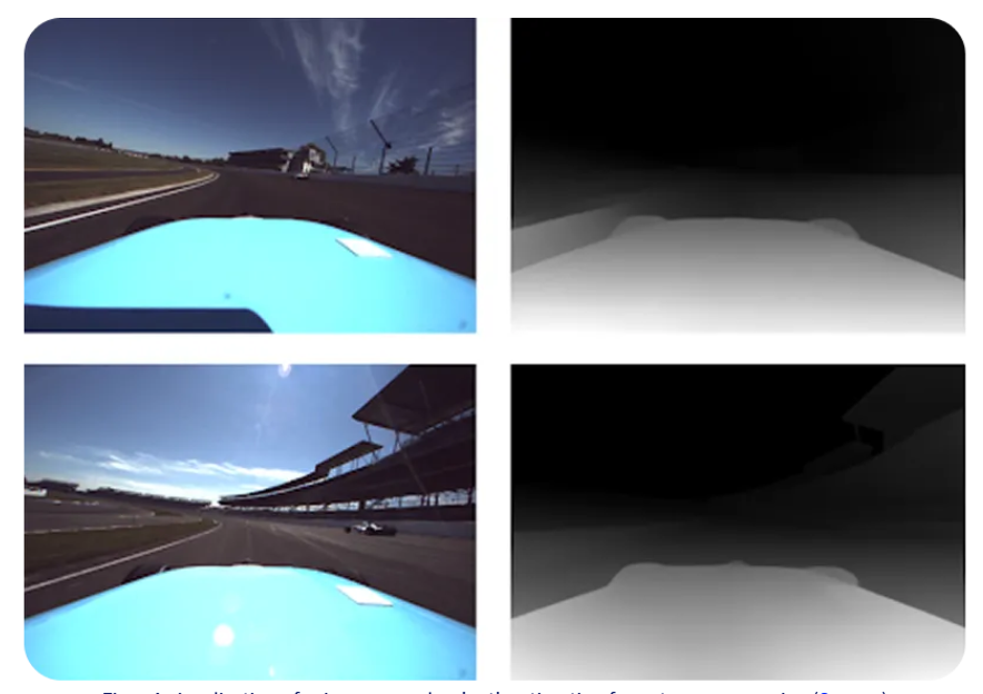AI Visual Insight: This image illustrates a 3D understanding scenario based on monocular RGB input. It highlights the reliance on depth priors, scene layout, and structural boundaries under single-view input, making it well suited to explain why monocular reconstruction requires learned depth estimation to compensate for missing absolute scale.

AI Visual Insight: This image shows a spatial recovery process driven by continuous video frames. It emphasizes the importance of inter-frame parallax, temporal continuity, and dynamic region handling, making it a good match for topics such as VO/SLAM, keyframe selection, and temporal consistency modeling.

modes = ["monocular", "multi_view", "video", "rgbd", "lidar"]

for mode in modes:
    if mode == "monocular":
        print("Prioritize monocular depth priors")  # Compensate for missing absolute scale
    elif mode == "multi_view":
        print("Prioritize learned MVS")  # Strengthen multi-view matching and fusion

This code snippet shows that different input modalities require different deep learning integration strategies.

Data capture quality is the first constraint on reconstruction quality

The most valuable investment during data capture is not direct 3D generation, but data governance. Blur, overexposure, redundant viewpoints, dynamic objects, and domain shift will all be amplified in later geometric stages, ultimately appearing as point cloud noise, depth discontinuities, and broken meshes.

You should prioritize three front-end capabilities: image quality assessment, keyframe selection, and dynamic region detection. Their shared objective is to ensure that the data entering the reconstruction pipeline is reconstructable, fusible, and trackable.

The quality gating layer should exist as a general-purpose front end

Online IQA can filter out defocused and exposure-abnormal frames. Keyframe selection reduces redundant data. Dynamic masks can reduce the damage caused by pedestrians and vehicles to static mapping. For mobile or robotic systems, this layer often delivers more value than upgrading the back-end model.

score = iqa_model(frame)          # Image quality score
is_dynamic = seg_model(frame)     # Dynamic region segmentation

if score > 0.8 and not is_dynamic.any():
    save_as_keyframe(frame)       # Keep only high-quality static keyframes

This code snippet describes how the capture front end can use lightweight models for real-time filtering.

The core goal of the geometric front end is to model cameras and poses reliably

Calibration, pose estimation, and multi-source registration form the geometric foundation of 3D reconstruction. The most effective use of deep learning here is not to replace PnP, BA, or ICP, but to improve feature stability, matching quality, and uncertainty modeling.

A typical combined paradigm is learned feature extraction + learned matching + geometric solving. This preserves interpretability while improving solvability in scenes with weak texture, low illumination, and large viewpoint changes.

Learning-based enhancement should serve geometric constraints rather than bypass them

In production practice, you should propagate confidence through the entire process of matching, solving, and optimization. Incorrect matches cannot be eliminated completely, but their damage can be significantly reduced through weighted PnP, robust-kernel BA, and cross-modal coarse registration.

matches = matcher(img1, img2)             # Learned matcher outputs candidate correspondences
inliers = geometric_verify(matches)       # Geometric verification removes outliers
pose = solve_pnp(inliers)                 # Solve camera pose from inliers

This code snippet summarizes the mainstream engineering path of learned matching + geometric verification + pose solving.

Depth estimation and multi-view geometry are the key bridge between front end and back end

The focus at this layer is not just to output depth maps, but to output depth + confidence + consistency results. Monocular depth works well as a prior, multi-view depth is responsible for primary geometry recovery, and geometric consistency filtering determines which results can truly enter the fusion stage.

Learned MVS, confidence prediction, and forward-backward reprojection checks are critical for controlling false depth, floating surfaces, and edge misalignment. Without this layer, it is difficult to stabilize the quality of subsequent point clouds and meshes.

Uncertainty must be modeled explicitly before fusion

Many systems fail not because the depth values are inaccurate, but because incorrect depth is averaged into the result with equal weight. The correct approach is to generate a probability or uncertainty value for each pixel, then map it to a fusion weight.

Dense reconstruction and representation generation should choose the right representation for the task

Point clouds are suitable for measurement and post-processing. Meshes are better for delivery and simulation. TSDF works well for real-time incremental mapping. Implicit fields are suitable for continuous surface representation. NeRF and 3DGS are better at high-fidelity novel view rendering. There is no single optimal representation—only the representation that best matches the business requirement.

In engineering practice, the most reliable pipeline is usually: generate point clouds through depth fusion, enhance the point clouds, extract meshes, and then convert them into implicit fields or neural representations when needed. This balances interpretability with visual quality.

Appearance recovery determines whether the result has product value

Correct geometry only means that the shape is right. Texture, material, and lighting recovery determine whether it actually looks right. Multi-view texture fusion, super-resolution enhancement, handling of reflective and transparent regions, and PBR material estimation are key steps for high-quality digital twins and content production.

Especially for reflective, transparent, or weak-texture objects, direct texturing often introduces false textures. A more reliable method is to perform material recognition and lighting decomposition first, then apply quality-weighted fusion.

Dynamic scenes and semantic enhancement are driving systems into real-world applications

The challenge of dynamic scene reconstruction is to satisfy both spatial consistency and temporal consistency at the same time. Static-dynamic decoupling, temporal depth smoothing, pose drift suppression, and 4D representations are core capabilities for video mapping, autonomous driving, and robotic inspection.

Semantic enhancement turns a 3D model from a geometric asset into a data asset that can be searched, edited, and used for decision-making. Mapping 2D segmentation into 3D, instance-level modeling, semantics-constrained geometric optimization, and open-vocabulary recognition directly increase the business value of reconstruction systems.

labels_2d = segmentor(image)                 # Generate 2D semantic labels
points_3d = back_project(depth, intrinsics)  # Back-project depth into 3D
semantic_map = fuse_semantics(points_3d, labels_2d)  # Fuse into a semantic point cloud

This code snippet demonstrates the basic mapping process from 2D semantics to a 3D semantic map.

Deliverable pipelines share the same traits: closed-loop operation and maintainability

A truly mature 3D reconstruction system must ultimately return to metrics, alerts, and deployment. At the front end, you should measure usable frame rate, coverage, and dynamic ratio. In the geometric front end, you should track inlier ratio, ATE, and RPE. In the back end, you should evaluate completeness, F-score, mesh quality, and rendering consistency.

Once the system supports quality gating, extrinsic drift alerts, semantic blind-spot warnings, and recapture recommendations, 3D reconstruction has truly evolved from a research prototype into an engineering system that can sustain long-term iteration.

FAQ

Q1: What deep learning module should be deployed first in a 3D reconstruction project?

A: Start with data capture governance, including image quality assessment, keyframe selection, and dynamic detection. These three modules are low-cost, high-return investments that directly improve the stability of the entire pipeline.

Q2: Can NeRF or 3DGS fully replace traditional SfM/MVS?

A: No. NeRF and 3DGS are better at appearance modeling and novel view synthesis, but geometry editability, deployment complexity, and system stability still require support from traditional geometric pipelines. In practice, hybrid approaches usually work best.

Q3: How can you tell whether a 3D reconstruction system is ready for production?

A: Check four things: whether the input can be governed, whether pose can be solved reliably, whether the output can be evaluated quantitatively, and whether the system has a closed loop for alerting and recapture. Only when all four are in place does the system have long-term delivery capability.

AI Readability Summary

This article reconstructs the full engineering chain of 3D reconstruction and systematically explains how deep learning enhances data capture, calibration and registration, depth estimation, dense reconstruction, appearance recovery, dynamic modeling, and semantic enhancement—forming a 3D reconstruction pipeline that balances accuracy, robustness, deployability, and maintainability.