This article focuses on exponential-function nonlinear regression and shows how to use Python, SciPy, and scikit-learn for data generation, parameter fitting, error evaluation, and noise experiments. It addresses a core practical challenge: how to fit and validate nonlinear models reliably. Keywords: nonlinear regression, curve_fit, exponential fitting.
Technical Specifications Snapshot
| Parameter | Description |
|---|---|
| Language | Python |
| Core Task | Exponential-function nonlinear regression |
| Fitting Method | Nonlinear least squares |
| Optimization Algorithm | Levenberg-Marquardt (lm) |
| Core Dependencies | NumPy, SciPy, Matplotlib, scikit-learn |
| Data Source | Simulated noisy samples |
| Star Count | Not provided in the original content |
| Use Cases | Growth modeling, decay modeling, experimental curve fitting |
This article fully explains how to fit an exponential function with nonlinear regression
Nonlinear regression is suitable when the relationship between the target variable and features is not linear. Unlike linear regression, which directly fits a straight line, nonlinear regression requires you to define the functional form first and then estimate parameters through an optimization algorithm.
This example uses the exponential model y = a * exp(bx) + c. Here, a controls amplitude, b controls the growth or decay rate, and c represents the overall offset. This type of model is common in population growth, chemical reactions, and sensor response analysis.
The exponential model should be defined explicitly first
import numpy as np

def exponential_func(x, a, b, c):
    # Exponential function model: amplitude a, growth rate b, offset c
    return a * np.exp(b * x) + c
This code converts the mathematical model into a Python function interface that an optimizer can use.
The simulated data generation stage determines whether the later fitting results are truly verifiable
To validate the algorithm properly, the safest approach is to construct a sample dataset with known ground-truth parameters. In the original example, the parameters are set to a=2.5, b=0.3, c=1.0, and Gaussian noise is added to simulate real measurement error.
This approach provides two clear benefits: first, you can directly compare the true parameters with the fitted parameters; second, it makes it easy to study how changing noise levels affect model robustness.
def generate_simulated_data(seed=42, n_samples=100, noise_level=0.05):
    # Fix the random seed to ensure reproducible experiments
    np.random.seed(seed)

    true_params = {"a": 2.5, "b": 0.3, "c": 1.0}
    x = np.linspace(0, 5, n_samples)
    y_true = exponential_func(x, **true_params)

    # Add Gaussian noise scaled by the maximum value of the true curve
    noise = np.random.normal(0, noise_level * np.max(y_true), n_samples)
    y_noisy = y_true + noise
    return x, y_true, y_noisy, true_params
This code generates reproducible exponential regression data with a controllable noise level.
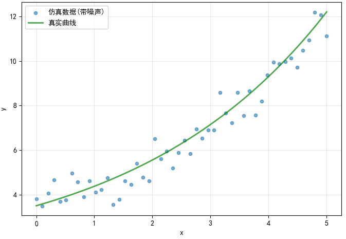 AI Visual Insight: The chart shows the overlay between the ideal exponential curve and noisy scatter points. The points fluctuate randomly around the curve, indicating that sample error mainly appears as amplitude perturbation rather than structural drift. That makes this dataset especially suitable for testing whether least-squares fitting can recover the exponential growth trend.
Nonlinear least squares is the core mechanism behind exponential regression
The objective is to minimize the sum of squared residuals between observed and predicted values, namely min Σ(y_i - ŷ_i)^2. Unlike linear regression, the parameters here appear inside the exponential term, so there is usually no direct analytical solution and numerical optimization is required.
SciPy’s curve_fit is one of the most common entry points for nonlinear fitting in Python. It performs an iterative search from an initial guess so that the model output gradually approaches the observed data.
Choosing a reasonable initial guess significantly improves convergence stability
from scipy.optimize import curve_fit

def fit_exponential_model(x, y, initial_guess=None):
    if initial_guess is None:
        # A heuristic initial guess can help the optimizer converge faster
        initial_guess = [1.0, 0.1, 0.0]

    params, covariance = curve_fit(
        exponential_func,
        x,
        y,
        p0=initial_guess,      # Initial parameter guess
        maxfev=10000,          # Increase the maximum number of function evaluations to avoid early stopping
        method='lm'            # Use the LM algorithm for least-squares optimization
    )

    # The square roots of the covariance diagonal can be interpreted approximately as parameter standard errors
    perr = np.sqrt(np.diag(covariance))
    return params, perr, covariance
This code uses curve_fit to estimate exponential-function parameters and approximate parameter uncertainty.
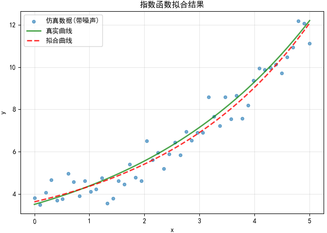 AI Visual Insight: The red dashed line closely matches the true exponential curve, which indicates that the fitted parameters successfully recover the overall growth shape. If local deviations are concentrated in the high-value region, that usually means the noise is being amplified by the exponential form, a common sign that exponential models become more sensitive in the tail.
A regression model must be evaluated with multiple metrics instead of the fitted curve alone
A visually good fit does not automatically mean the model is reliable. In practice, you should evaluate at least four metrics together: R², MSE, RMSE, and MAE. R² measures explanatory power, MSE and RMSE quantify squared-error magnitude, and MAE measures the average absolute deviation.
Among them, RMSE is easier to interpret because it uses the same unit scale as the original data. MAE is also less sensitive to outliers than MSE, which makes it useful for assessing overall robustness.
from sklearn.metrics import r2_score, mean_squared_error, mean_absolute_error

def evaluate_fit(y_true, y_pred):
    r2 = r2_score(y_true, y_pred)
    mse = mean_squared_error(y_true, y_pred)
    rmse = np.sqrt(mse)      # Convert squared error back to the original unit scale
    mae = mean_absolute_error(y_true, y_pred)
    return {"R2": r2, "MSE": mse, "RMSE": rmse, "MAE": mae}
This code returns a standard set of regression metrics that you can use directly in reports and comparisons.
Residual distributions reveal whether the model has actually learned the pattern
If residuals are randomly distributed around zero, the model structure is usually appropriate. If the residuals show a trend, fan-shaped spread, or periodic pattern, that often indicates model misspecification or heteroscedasticity.
In the original example, the residual plot is mostly scattered randomly around the zero line with no obvious systematic bias. That suggests the exponential structure matches the underlying data-generation process.
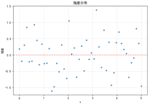 AI Visual Insight: The residual cloud is distributed approximately symmetrically around the zero reference line, with no obvious curved band or drift trend. This suggests the model is not missing any major nonlinear structure. If dispersion increases slightly at higher
 x values, that may reflect how the absolute noise magnitude grows as the exponential values become larger.
Noise experiments can directly validate the model’s robustness boundary
noise_levels = [0.01, 0.05, 0.1, 0.2]
r2_scores = []

for i, noise in enumerate(noise_levels):
    x, y_true, y_noisy, _ = generate_simulated_data(
        seed=1000 + i,
        n_samples=50,
        noise_level=noise
    )
    params, _, _ = fit_exponential_model(x, y_noisy, [1.0, 0.2, 0.0])
    y_pred = exponential_func(x, *params)
    r2_scores.append(evaluate_fit(y_true, y_pred)["R2"])
This code quantifies how the explanatory power of exponential regression changes under different noise levels.
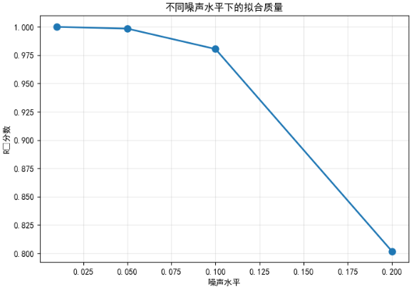 AI Visual Insight: The chart shows
 R² decreasing as the noise level rises. The trend is smooth and statistically expected, indicating that the current fitting workflow remains stable under low-noise conditions but loses explanatory power significantly in high-noise regimes. This kind of curve is useful for defining an acceptable noise threshold for the model.
This case shows that the engineering value of exponential regression lies in interpretability and verifiability
The main strengths of this method are its clear structure, interpretable parameters, and low implementation cost. For tasks where the underlying process is known to approximately follow an exponential law, curve_fit is often more efficient than forcing a more complex model.
However, it also has clear limits. Poor initial guesses can prevent convergence, large noise can make parameter estimates unstable, and if the true pattern is not exponential, forcing this fit will distort error interpretation. That is why residual analysis and noise experiments are not optional extras; they are required steps.
FAQ: The three questions developers care about most
Q1: Why does nonlinear regression depend more on initial values than linear regression?
Because nonlinear optimization usually has no analytical solution, the solver depends on iterative search toward a local optimum. If the initial guess is too far from the true parameters, convergence may be slow, get trapped in a local optimum, or fail entirely.
Q2: When should you prioritize using curve_fit?
When you already know the function form—such as an exponential, power-law, or logistic curve—and your goal is to estimate a small number of interpretable parameters, curve_fit is the most direct and lightweight choice.
Q3: If R² is very high, does that mean the model is definitely usable?
Not necessarily. A high R² only indicates strong explanatory power. It does not prove that the residuals are unbiased, the parameters are stable, or the model structure is correct. You still need to evaluate the residual plot, MAE/RMSE, and noise sensitivity together.
Core summary
This article uses an exponential function to reconstruct the full nonlinear regression workflow: define the model, generate simulated data with noise, use SciPy curve_fit for least-squares fitting, evaluate the results with R², MSE, RMSE, MAE, and residual analysis, and finally explain how noise level affects fitting quality.