Multi-UAV Cooperative Transport Path Planning and Dynamic Control: A Matlab Implementation with 3D RRT, Dual-UAV Handover, and EKF Payload Mass Estimation - Devuly | Smart Analytics for Developers & Projects

This project focuses on cooperative multi-UAV payload transport. It integrates 3D RRT obstacle avoidance, synchronized dual-UAV handover, and EKF-based payload mass estimation to address path generation, coordinated switching, and limited control accuracy under unknown payload conditions in complex environments. Keywords: multi-UAV cooperation, 3D RRT, dynamic mass estimation.

Table of Contents

Technical Specifications Snapshot

Parameter	Description
Primary Language	Matlab
Simulation Environment	Unity 3D + Matlab
Core Algorithms	3D RRT, PID, EKF, seventh-order polynomial trajectory smoothing
Task Type	Dual-UAV cooperative pickup, transport, and handover
Obstacle Modeling	Static walls/cylinders + dynamic obstacles
Code Structure	Hybrid of research scripts and function calls
GitHub Stars	Original data not provided
Core Dependencies	Matlab numerical computing, collision detection modules, RRT functions

This solution uses a hierarchical control framework for cooperative transport research

The original project represents a typical research-grade simulation workflow: two UAVs complete target pickup, cooperative transport, and payload handover in a 3D obstacle environment. Its value does not come from any single algorithm, but from the end-to-end integration of planning, control, and estimation into a closed loop.

The system addresses three core pain points: obstacle avoidance in complex 3D space, timing synchronization during dual-UAV handover, and controller parameter mismatch caused by unknown payload mass. This implementation handles them with 3D RRT, a distance-triggered synchronization mechanism, and online EKF mass estimation, respectively.

The system uses a layered architecture to decompose task complexity

The upper layer splits the mission into stages such as takeoff, target approach, pickup, transport, handover, and release. The middle layer generates executable paths in obstacle-filled space. The lower layer handles trajectory tracking, attitude stabilization, and thrust allocation.

This structure keeps module boundaries clear. You can replace path planning with RRT* or PRM, and you can upgrade the controller from PID to MPC, without breaking the overall mission flow.

for GENERAL = 1:3
    start = travel(GENERAL,1:3);   % Read the start point of the current stage
    goal  = travel(GENERAL,4:6);   % Read the goal point of the current stage

    % Call RRT to generate an obstacle-avoiding path
    [NODELIST, PATH, COORD_PATH, found] = RRT(start, goal, a, ...
        meshes_vector, delta, check_line, range_goal);

    TOTAL_COORD_PATH = [TOTAL_COORD_PATH; COORD_PATH]; % Concatenate the global path
end

This code plans the 3D path stage by stage and merges the results into a globally executable flight route.

3D RRT generates feasible paths quickly in obstacle-constrained space

RRT is not designed to find the globally optimal path first. Its strength is finding a path that is safe and flyable as quickly as possible. For cooperative multi-UAV transport, obtaining a safe route matters more than optimizing for path length at the beginning.

In the original parameter set, delta controls the tree expansion step size, range_goal determines whether a new node has entered the goal neighborhood, and check_line defines the collision-checking sampling density along line segments. Together, these parameters determine the trade-off between planning speed and safety.

Trajectory smoothing uses a seventh-order polynomial to reduce flight jitter

Raw RRT output usually contains piecewise linear segments with sharp corners, which makes it unsuitable for direct execution by a flight controller. This implementation uses a seventh-order polynomial to generate smooth inter-segment trajectories, improving continuity in velocity, acceleration, and even jerk boundaries, and reducing abrupt attitude changes.

A = [1 0 0 0 0 0 0 0;
     1 1 1 1 1 1 1 1;
     0 1 0 0 0 0 0 0;
     0 1 2 3 4 5 6 7;
     0 0 2 0 0 0 0 0;
     0 0 2 6 12 20 30 42;
     0 0 0 6 0 0 0 0;
     0 0 0 9 24 60 120 210];

b = [0 1 des_vel_0 des_vel_1 des_acc_0 des_acc_1 des_jerk_0 des_jerk_1]';
ai = A \ b;   % Solve for the seventh-order polynomial coefficients

This code constructs a smooth time-scaling function from boundary constraints on position, velocity, acceleration, and jerk.

The dual-UAV synchronization mechanism determines whether handover remains stable and reliable

The real challenge in cooperative transport is not single-UAV flight, but maintaining a shared mission state across two UAVs in space. This implementation uses the distance threshold dsync as the handover trigger. When the two UAVs move within the specified range, the first UAV releases the payload and the second UAV takes over.

This strategy is simple and effective from an engineering perspective, but it is still fundamentally an event-triggered synchronization method. If communication delay, velocity mismatch, or wind disturbance exists, a distance threshold alone may not be enough. The lower-level error compensation controller must work with it.

Payload switching logic reduces control transients through mass inheritance

During the transport phase, the first UAV continuously estimates payload mass. Once the system enters the handover zone, the second UAV directly inherits the final estimated mass value instead of restarting from an initial guess. This avoids insufficient thrust or attitude overshoot during the handover instant.

if distance_uav < dsync
    release_flag = 1;              % The first UAV performs the release
    pickup_flag_uav2 = 1;          % The second UAV starts pickup
    m_est_uav2 = m_est_uav1;       % Inherit the final mass estimate
end

This pseudocode expresses the core control logic of the handover stage: state triggering, action switching, and parameter inheritance.

Online EKF mass estimation improves control accuracy under unknown payload conditions

Unknown mass is a key source of uncertainty in cooperative transport. If the controller is always designed around a fixed mass, thrust and attitude regulation will remain biased, especially after pickup.

The EKF treats mass as an estimated state and updates it jointly with velocity, acceleration, and sensor observations. As a result, the controller receives a continuously refined online estimate rather than a static nominal value.

AI Visual Insight: This figure shows the state update equations of the Extended Kalman Filter, including the prior estimate, Kalman gain, and measurement residual. It illustrates how sensor observation errors feed back into mass-state correction and provides the mathematical foundation for online unknown-payload estimation.

Mass estimation feeds directly into the thrust allocation equation

The thrust model follows F = m * (g + a). Once m changes from a fixed value to a real-time estimate, the controller can compensate for payload variation more accurately and reduce lag during ascent as well as oscillation during handover.

Simulation results show strong value for reproducible research

The reported results include an average path planning time of about 2.3 seconds, handover position error below 0.5 meters, synchronization time under 3 seconds, and EKF convergence to near the true mass within 10 seconds. These results suggest that the approach is practical and reproducible in research-oriented simulation.

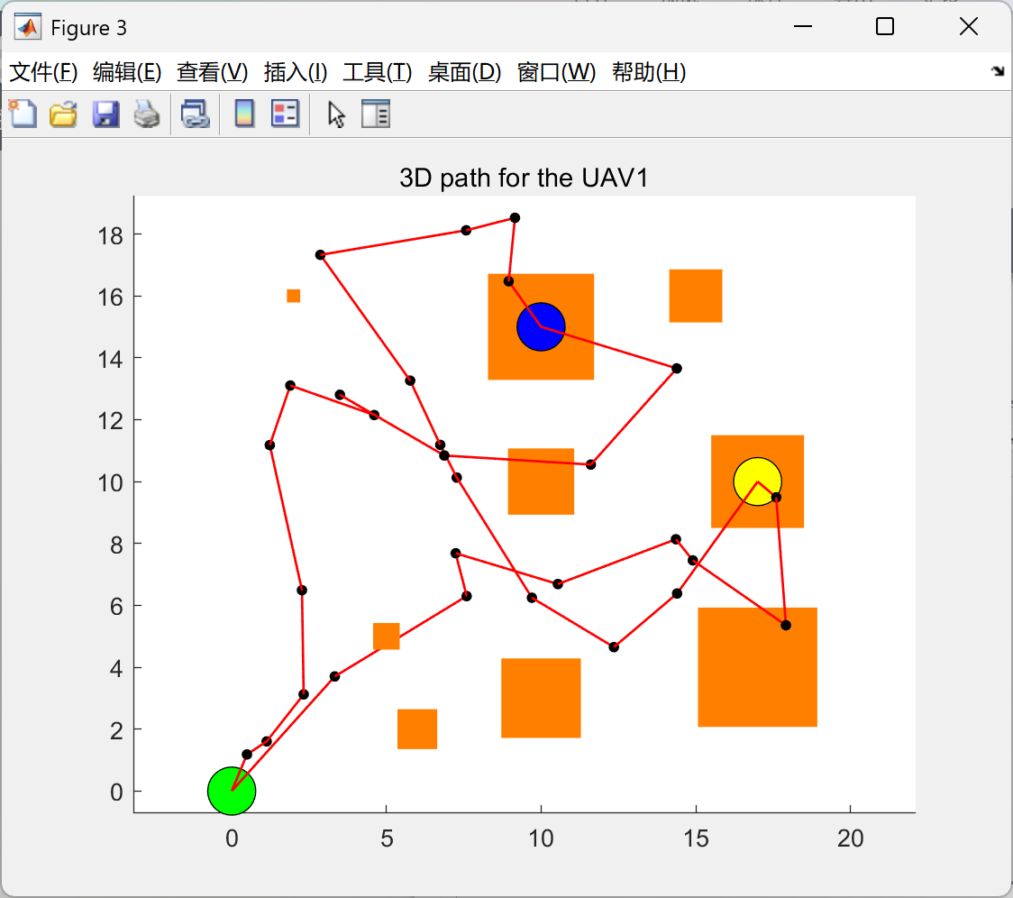
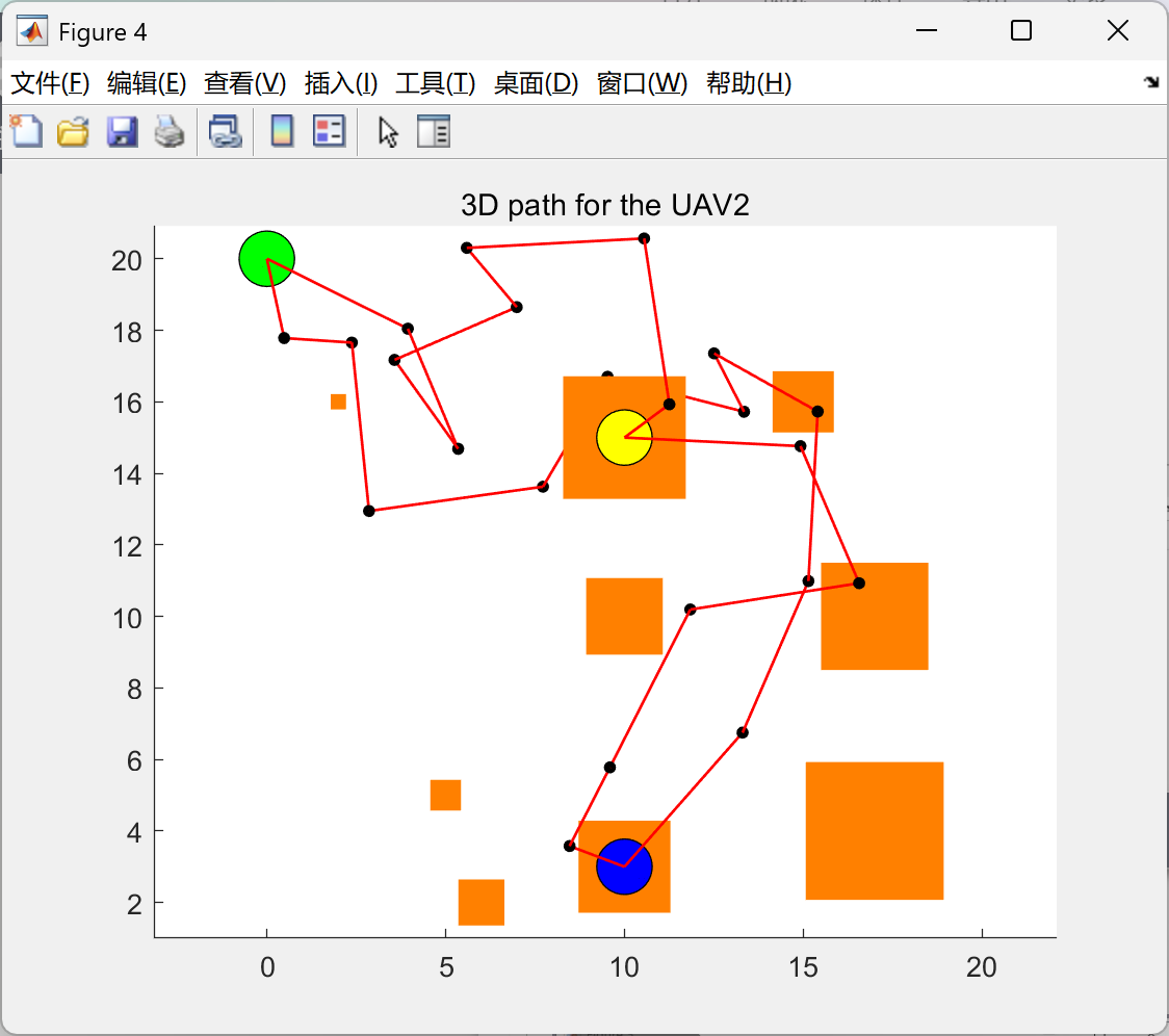
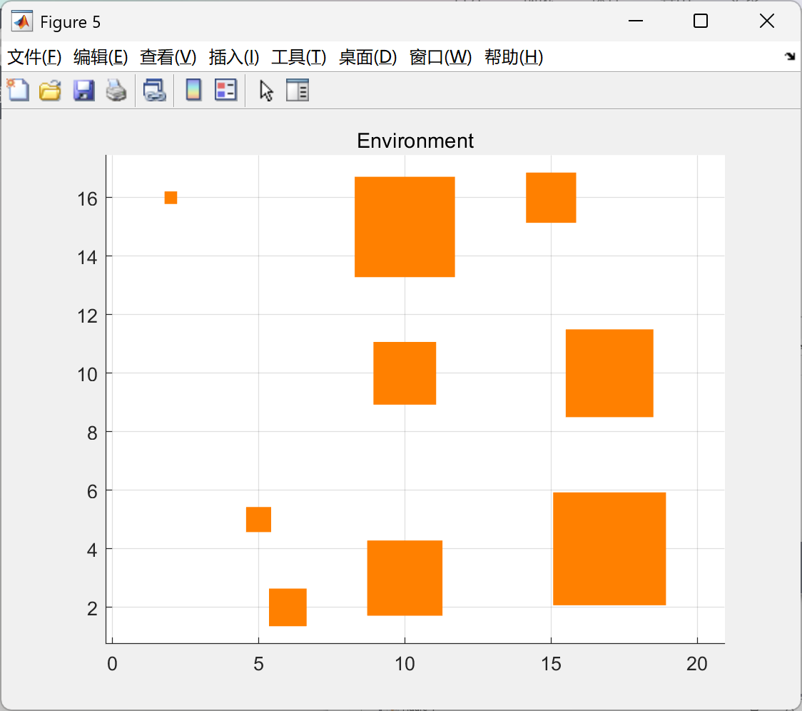
AI Visual Insight: This figure likely shows the initial trajectory or obstacle distribution in a 3D scene, including the start and goal positions, obstacle volumes, and the RRT expansion tree, helping validate reachability and obstacle avoidance effectiveness in complex space.

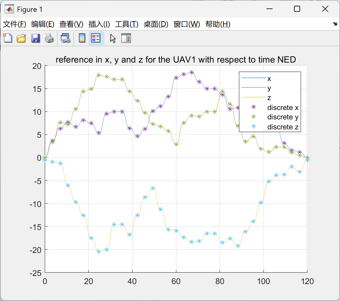
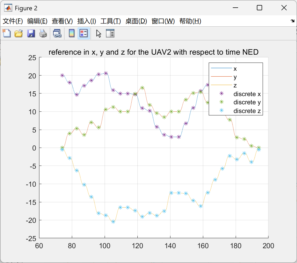AI Visual Insight: This figure likely presents the smoothed trajectory after path post-processing. Compared with the original polyline path, it appears more continuous and helps visualize reduced curvature and lower attitude-control burden.

AI Visual Insight: This figure is typically used to show the spatial relationship between the two UAVs during cooperation, with emphasis on the handover zone, relative distance, and synchronization trigger timing to verify the stability of the coordination mechanism.

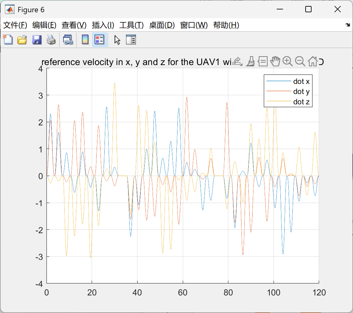
AI Visual Insight: This figure likely shows attitude, position, or velocity tracking curves and is useful for evaluating overshoot, steady-state error, and convergence speed before and after payload variation.

AI Visual Insight: This figure likely shows how the mass estimate converges toward the true value over time. If the curve oscillates before settling, it indicates that the EKF has a degree of robustness to observation noise.

AI Visual Insight: This figure most likely corresponds to thrust or control input variation and can be used to evaluate whether control commands remain smooth or exhibit abrupt changes at pickup and handover events.

This approach still leaves three clear paths for engineering upgrades

First, RRT is suitable for finding feasible solutions, but path quality is often limited. If your objective shifts toward energy efficiency or time optimality, consider upgrading to RRT, Informed RRT, or a hybrid path optimization pipeline.

Second, local replanning is still relatively passive. In the presence of dynamic obstacles and multi-UAV interaction, a receding-horizon controller or predictive collision-avoidance framework is better suited for true online closed-loop planning.

Third, the current dual-UAV coordination behaves more like sequential relay transport than tightly coupled cooperative carrying. To handle flexible cables, suspended-load swing, or shared load-bearing, you should introduce explicit payload dynamics modeling.

for i = 1:size(TOTAL_COORD_PATH,1)-1
    % Map discrete path points into smooth trajectory segments
    new_piece = s_t' * (TOTAL_COORD_PATH(i+1,:) - TOTAL_COORD_PATH(i,:)) ...
              + TOTAL_COORD_PATH(i,:);
    PATH_TL = [PATH_TL; new_piece]; % Generate the complete time-parameterized trajectory
end

This code interpolates discrete path nodes into a continuous trajectory, bridging the gap between a path that can be planned and one that can actually be controlled.

FAQ

Which research scenarios is this project best suited for?

It is well suited for multi-UAV cooperative control, 3D path planning, unknown payload estimation, and Matlab-based simulation reproduction. It is especially useful as a graduate course project or a baseline for algorithm comparison.

Why is trajectory smoothing necessary after RRT?

Because RRT outputs a discrete polyline path with abrupt corner transitions. Flight controllers need reference trajectories with continuous velocity and acceleration. Seventh-order polynomial smoothing significantly reduces control jitter.

What direct value does EKF mass estimation provide for cooperative transport?

It updates the thrust model in real time when payload mass is unknown, allowing the UAVs to maintain more stable attitude and altitude control during pickup, transport, and handover while reducing cumulative error caused by parameter mismatch.

Core Summary: This article reconstructs a cooperative multi-UAV transport solution that uses 3D RRT for path planning in obstacle environments, hierarchical control for dual-UAV handover and trajectory tracking, and online EKF estimation for unknown payload mass. It is well suited for research reproduction, simulation validation, and cooperative control algorithm benchmarking.