This article focuses on cooperative multi-UAV payload transport. Its core contribution is the integration of 3D RRT path planning, dual-UAV handover synchronization, and EKF-based mass estimation into a single Matlab simulation framework to address obstacle avoidance in complex environments, control mismatch under unknown payloads, and coordination error during handover. Keywords: multi-UAV cooperation, 3D RRT, EKF payload mass estimation.
Technical Specifications at a Glance
| Parameter | Description |
|---|---|
| Primary Language | Matlab |
| Simulation Environment | Matlab + Unity |
| Core Algorithms | 3D RRT, EKF, PID, seventh-order polynomial trajectory smoothing |
| Task Type | Cooperative multi-UAV transport |
| Scenario Characteristics | 3D obstacle environments, static/dynamic obstacles |
| Star Count | Not provided in the source data |
| Core Dependencies | RRT path search, collision detection, trajectory interpolation, mass estimator |
The solution uses a layered control architecture to reduce the complexity of cooperative transport systems
The value of the original design does not lie in any single algorithm, but in how the full system is assembled. It separates task planning, path planning, and low-level control into independent layers, allowing the multi-UAV transport problem to be solved step by step instead of through one tightly coupled global optimization process.
The task-planning layer handles phase transitions such as pickup, transport, and handover. The path-planning layer generates flyable paths in 3D obstacle space. The low-level control layer performs trajectory tracking based on real-time state feedback and dynamically compensates for unknown payloads.
Minimal execution flow for layered control
stage = "pickup";              % Current task phase: pickup
path = planRRT3D(start, goal);  % Path-planning layer: generate an obstacle-avoiding path
mass_hat = 3.0;                 % Initial payload mass estimate

while ~mission_done
    state = getUAVState();      % Read UAV state
    mass_hat = ekfUpdate(state);% Update mass estimate online
    u = trackController(path, state, mass_hat); % Compute control input using estimated mass
    sendControl(u);             % Send control command
end
This code snippet shows the responsibility boundaries among the task layer, planning layer, and control layer.
3D RRT generates executable obstacle-avoiding paths in complex environments
RRT is well suited for fast feasible path search in high-dimensional continuous spaces. In cooperative transport scenarios, it prioritizes solving the practical problem of “getting there first,” then improves trackability through smoothing. This makes it more engineering-oriented than directly pursuing a globally optimal path.
In the original implementation, the key parameters include the iteration count, expansion step size, goal radius, and the number of sampled points used for line-segment collision checking. Together, these parameters determine search speed, path density, and collision-safety margin.
Core RRT parameter configuration snippet
a = 4000;          % Number of internal RRT iterations

delta = 5;         % Tree expansion step size
range_goal = 3;    % Goal proximity radius
check_line = 5;    % Number of samples for line collision checking

[NODELIST, PATH, COORD_PATH, found] = RRT(start, goal, a, ...
    meshes_vector, delta, check_line, range_goal); % Generate an obstacle-avoiding path
This code defines the convergence efficiency of the RRT search and the granularity of its safety checks.
Seventh-order polynomial smoothing converts a discrete path into a trackable trajectory
RRT typically outputs a polyline path. Using it directly for flight control can cause abrupt attitude changes. The original solution therefore applies a seventh-order polynomial to interpolate each path segment, ensuring continuity in position, velocity, acceleration, and even jerk at the boundary conditions.
This type of smoothing strategy is well suited for transport tasks because trajectory discontinuities can significantly amplify payload swing and synchronization error when carrying suspended loads or performing cooperative transport.
numpts_for_segment = 1000;      % Number of interpolation points per trajectory segment
lin = linspace(0,1,numpts_for_segment);
A = [1 0 0 0 0 0 0 0;
     1 1 1 1 1 1 1 1;
     0 1 0 0 0 0 0 0;
     0 1 2 3 4 5 6 7;
     0 0 2 0 0 0 0 0;
     0 0 2 6 12 20 30 42;
     0 0 0 6 0 0 0 0;
     0 0 0 9 24 60 120 210];   % Trajectory boundary constraint matrix
b = [0 1 0 0 0 0 0 0]';
ai = A\b;                       % Solve for polynomial coefficients
This code is used to generate trajectory interpolation coefficients that satisfy high-order continuity constraints.
The dual-UAV synchronization mechanism determines whether handover remains stable and reliable
The real challenge in cooperative transport is not single-UAV obstacle avoidance, but spatiotemporal consistency between two UAVs at the handover point. The original scheme uses a distance-threshold trigger strategy: when the distance between the two UAVs falls below a synchronization threshold, the first UAV releases the payload and the second UAV takes over.
This mechanism is simple but effective. Its main advantage is low implementation cost, which makes it suitable for rapid validation in Matlab simulations. Its downside is sensitivity to localization error and communication delay, so it must be paired with PID-based compensation or consensus-style coordination control.
Example handover trigger logic
d_sync = 1.0;                           % Synchronization trigger distance threshold
if norm(uav1_pos - uav2_pos) < d_sync   % When the two UAVs are close enough
    releasePayload();                   % The first UAV releases the payload
    startPickupByUAV2();                % The second UAV takes over
end
This code expresses the minimal decision logic for dual-UAV handover.
EKF payload mass estimation enables the controller to adapt to unknown load changes
Unknown payload mass directly affects thrust allocation and attitude control. If the system continues to assume a fixed mass model, tracking error can increase, handover can become unstable, and overshoot may occur. The original design uses an EKF to estimate mass online and resolve this model-mismatch problem.
The estimator uses sensor observations, kinematic states, and the thrust relationship to dynamically correct the mass parameter. As a result, the low-level controller can recompute control actions using the latest mass estimate and effectively “correct while flying.”
 AI Visual Insight: This figure shows the core structure of the EKF state-update equations, including the prediction residual and Kalman-gain correction terms. It illustrates how the system recursively updates the payload mass parameter by fusing observations with prior estimates, making it suitable for transport scenarios with unknown mass or modeling uncertainty.
F = mass_hat * (g + acc_cmd);   % Compute required thrust using the estimated mass
att_ref = attitudeFromForce(F); % Infer the attitude reference from thrust
u = pidTrack(att_ref, state);   % Closed-loop attitude control
This code shows how mass estimation directly enters the thrust and attitude-control pipeline.
Experimental results indicate reproducible engineering plausibility in simulation
The key metrics reported in the source data include an average planning time of about 2.3 seconds, handover position error below 0.5 meters, synchronization time under 3 seconds, and EKF convergence to the true mass within about 10 seconds, with steady-state error below 0.2 kilograms.
These results suggest that although the system remains at the simulation-validation stage, it already covers the three core challenges in multi-UAV transport: path feasibility, handover synchronization, and payload adaptivity.
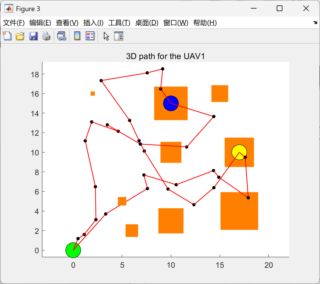
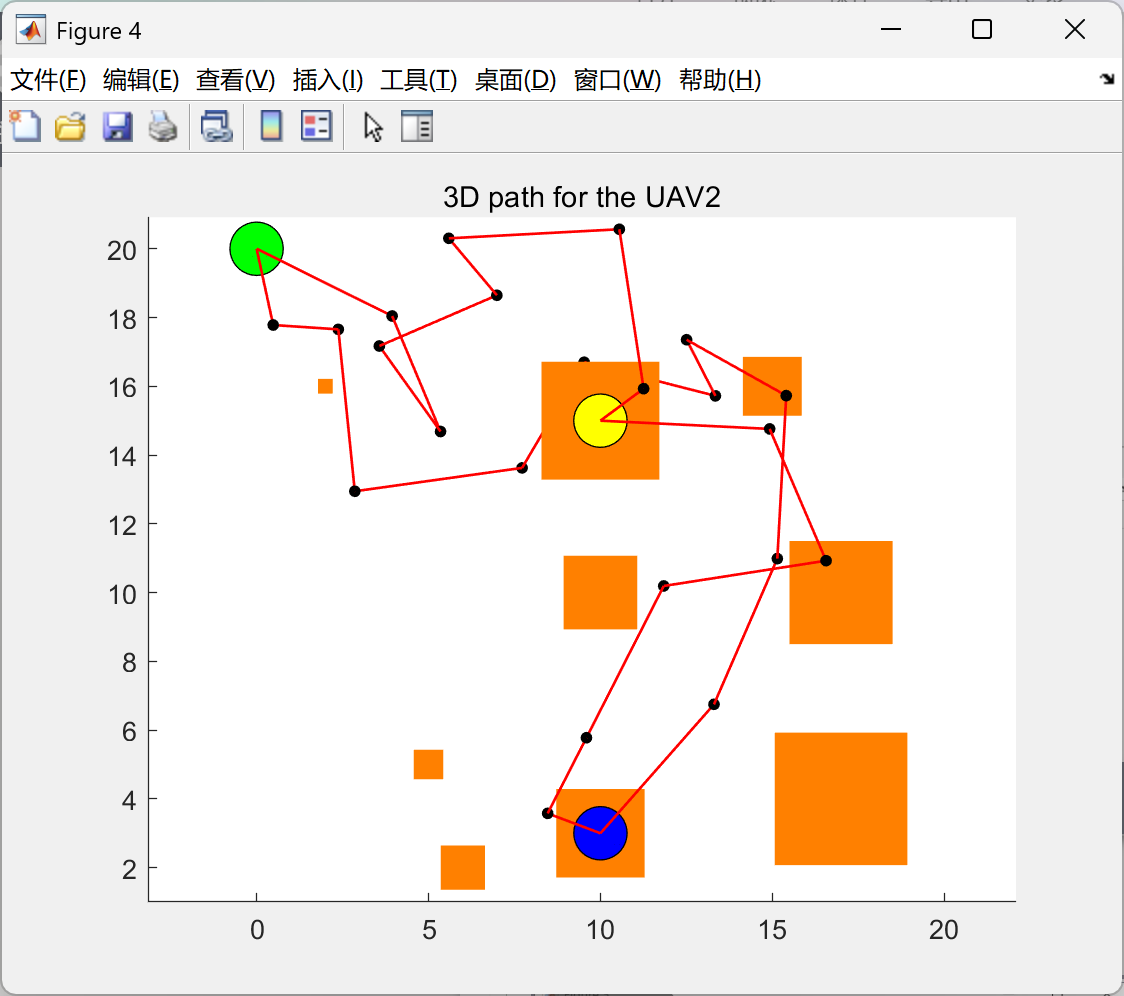
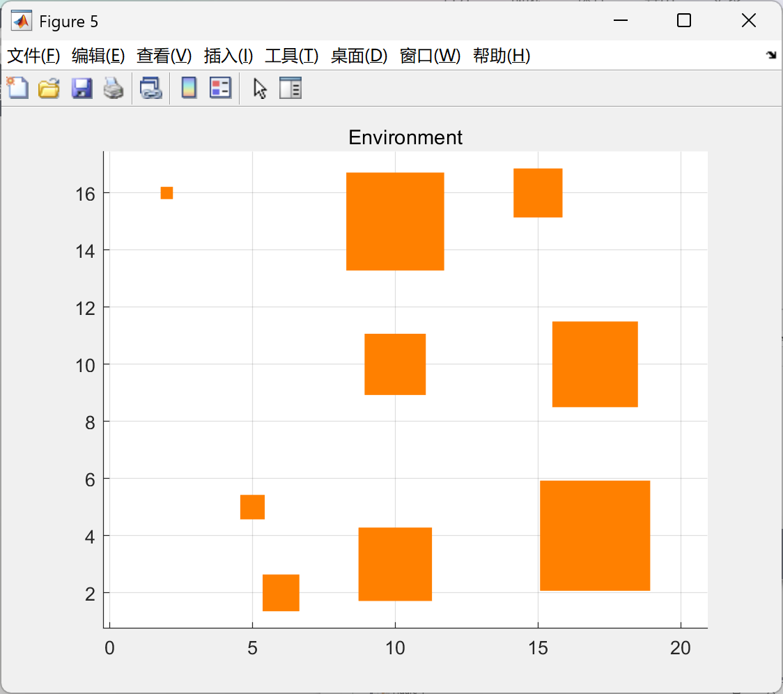
 AI Visual Insight: This figure most likely shows the overall trajectory distribution in a 3D environment. It can be used to assess whether the RRT-generated path successfully avoids obstacle regions and whether there are obvious detours or local redundancies between trajectory segments.
 AI Visual Insight: This figure may show a single-stage or local path-planning result. It is useful for inspecting node expansion density, path connectivity, and convergence behavior near the target point.
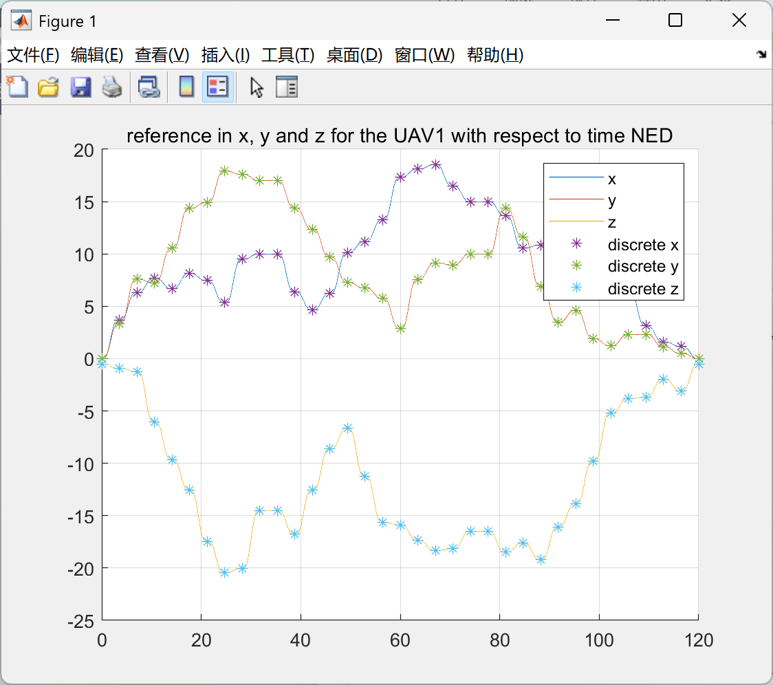
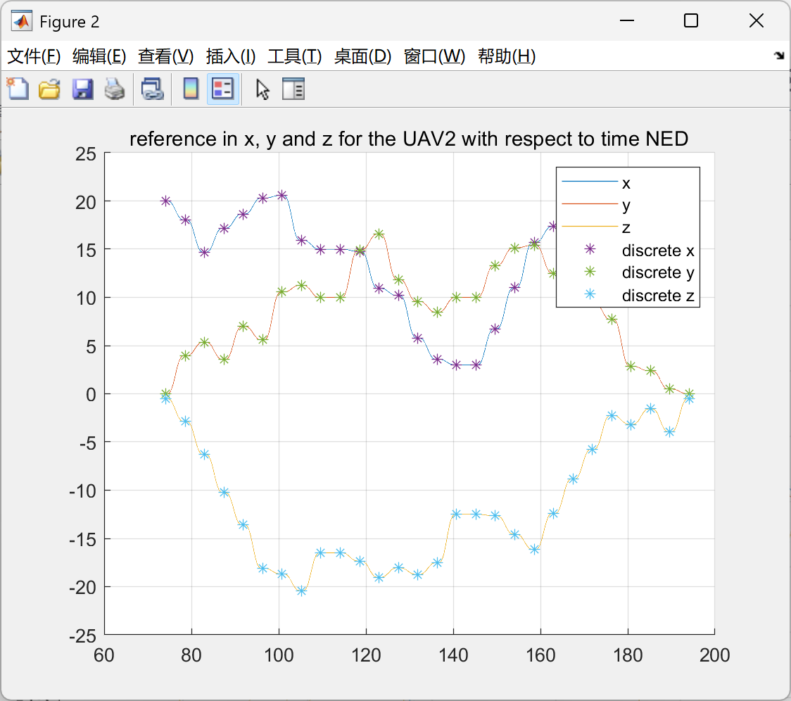
 AI Visual Insight: This figure may reflect the smoothed flight trajectory. Compared with the original polyline path, it appears more continuous and can help verify whether seventh-order polynomial interpolation reduces curvature discontinuities.
 AI Visual Insight: This figure may show the relative position changes of the two UAVs in the handover zone and can be used to determine whether the threshold-based synchronization strategy is sufficient to guarantee takeover accuracy.
 AI Visual Insight: This figure may correspond to attitude, velocity, or position tracking error curves and is useful for analyzing how payload changes affect controller stability.
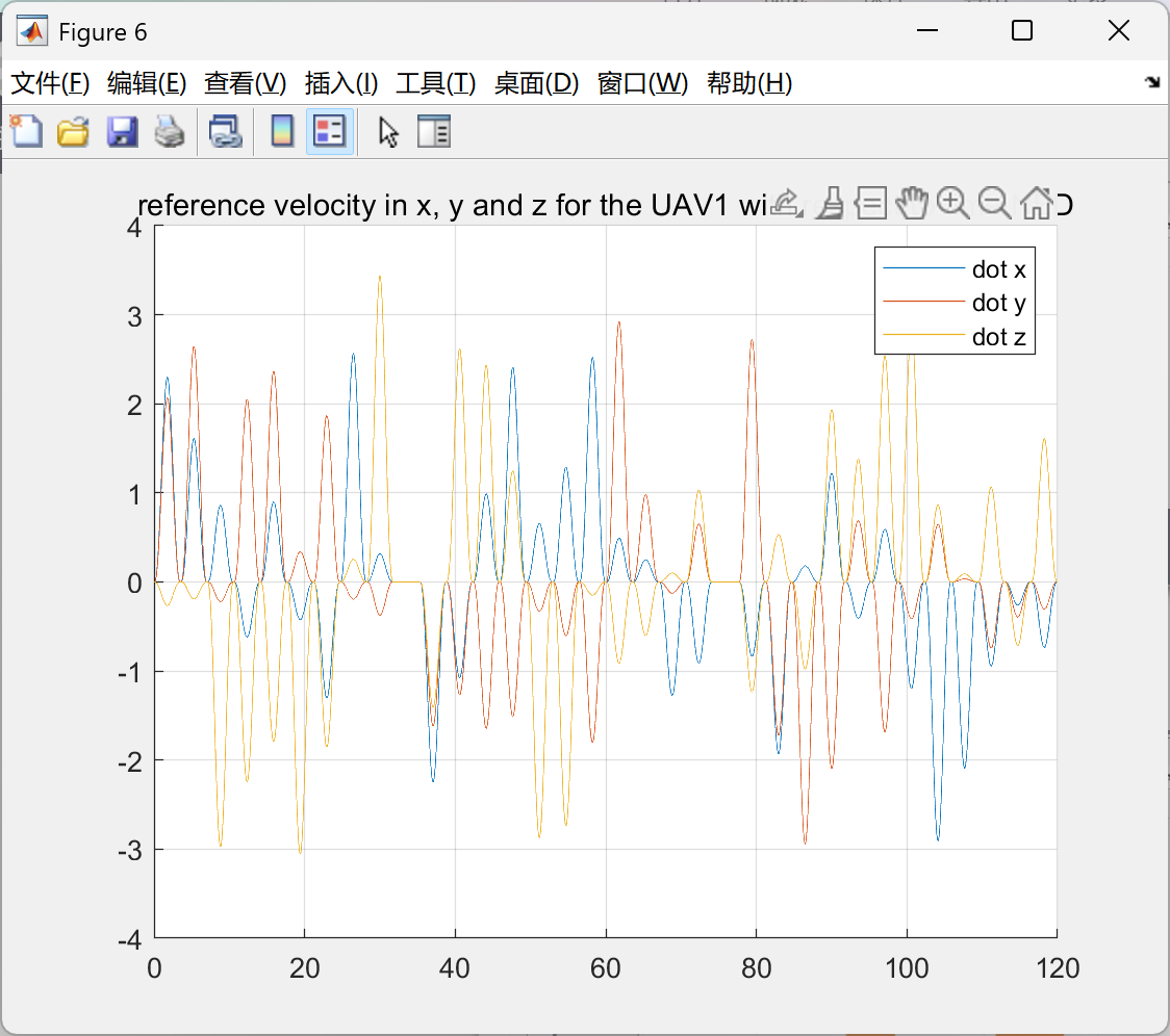 AI Visual Insight: This figure may show control inputs or thrust allocation over time, helping assess whether control effort becomes more stable after EKF-based mass estimation.
The solution still has three clear engineering upgrade paths
First, the path planner can be upgraded from RRT to RRT* or PRM to shorten path length and improve global path quality. Second, online replanning and receding-horizon control can be introduced to handle dynamic obstacles and inter-UAV collision avoidance. Third, the Unity visualization can be upgraded into a higher-fidelity digital-twin demonstration.
For real-world flight deployment, the system should also incorporate communication-delay modeling, rope or rigid-link payload dynamics, wind-disturbance modeling, and multi-UAV consensus control. Otherwise, a significant gap will remain between simulation and physical flight.
FAQ
1. Why choose RRT over A* in this case?
RRT is better suited to continuous 3D space and high-degree-of-freedom aerial vehicles, and it can quickly find feasible paths in complex obstacle environments. A* depends more heavily on discrete grids, and in 3D its computational and memory costs become much higher.
2. What problem does EKF payload mass estimation solve in cooperative transport?
It solves the model-mismatch problem caused by unknown payload mass. The controller can update thrust and attitude parameters based on the real-time mass estimate, thereby reducing tracking error and instability during handover.
3. What is still missing before this Matlab solution can be deployed on real UAVs?
It still lacks sensor-noise calibration, flight-controller interface integration, communication-delay compensation, dynamic-model identification, wind-field disturbance testing, and hardware-in-the-loop validation. These steps determine whether the algorithm can move from simulation to real flight.
Core Summary
This article reconstructs a cooperative multi-UAV payload transport solution: it organizes the mission flow with a layered control architecture, uses 3D RRT for obstacle-avoiding path planning, enables handover through a dual-UAV synchronization mechanism, and estimates unknown payload mass online with an EKF. The framework is well suited for Matlab-based simulation and algorithm validation.