WSN Coverage Hole Recovery with Q-Learning and Game Theory: A MATLAB Simulation Guide

This article explains a hybrid algorithm for wireless sensor network coverage hole recovery. It models multi-node coordination with a potential game and learns movement and sensing-radius adjustment strategies with Q-Learning, improving coverage while suppressing energy consumption and redundant overlap. Keywords: WSN, Q-Learning, Game Theory.

Technical specifications define the simulation scope

Parameter	Value
Primary Language	MATLAB
Application Domain	Wireless Sensor Network Coverage Recovery
Learning Paradigm	Reinforcement Learning (Q-Learning)
Coordination Mechanism	Potential Game
Network Size	30 sensor nodes
Failed Nodes	12
Number of Actions	9
Number of Discrete States	12
Communication Range	35 m
Sensing Radius Range	10 m – 20 m
Training Episodes	1000
Core Dependencies	MATLAB 2024b, matrix operations, grid-based coverage evaluation
Stars	Not provided in the source data

This method addresses the classic problem of WSN coverage hole recovery

After deployment, nodes in a wireless sensor network often fail because of energy depletion, hardware damage, or environmental impact. The result is not just a disconnected node. It creates unobservable coverage blind spots in the monitored area.

Traditional methods usually choose one of two options: move nodes to fill holes, or enlarge the sensing radius to compensate. The first offers stronger recovery capability but incurs higher mobility cost. The second is easier to implement but increases energy consumption and coverage overlap.

The core idea of the hybrid strategy is to turn hole recovery into a distributed decision problem

This approach treats each surviving node as an autonomous agent. Instead of depending on a global controller, each node decides from local state information whether to move, where to move, and whether to adjust its sensing radius.

Compared with static heuristic methods, reinforcement learning can continuously improve through trial and error in dynamic environments. Compared with pure reinforcement learning, game theory further constrains coordination among multiple nodes and reduces duplicate coverage caused by isolated decisions.

% --- Network parameters ---
area_W = 100;          % Area width
area_H = 100;          % Area height
num_sensors = 30;      % Total number of sensors
num_fail = 12;         % Number of failed nodes
r_sense_init = 15;     % Initial sensing radius
R_comm = 35;           % Communication range

grid_res = 2;          % Grid resolution for coverage evaluation
move_step = 2.5;       % Single-step node movement distance
range_step = 1.0;      % Sensing radius adjustment step

These parameters define the physical boundary conditions, network scale, and action granularity of the simulation. They form the basis for the later coverage recovery experiments.

The coverage model first defines how a hole is quantified

Within a 2D monitoring area, nodes cover grid points under a Boolean sensing model. If a region is not covered by any valid node, or its coverage level falls below a threshold, it is treated as a coverage hole.

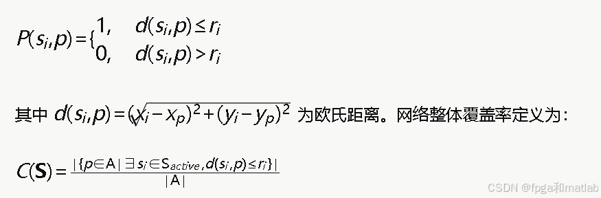AI Visual Insight: This figure shows the single-node coverage decision expression under the Boolean sensing model. The key idea is that coverage depends on whether the Euclidean distance between a node and a target point is smaller than the sensing radius. This serves as the mathematical basis for later global coverage computation and hole detection.

This definition is critical because the later reward function, state discretization, and policy updates all rely on the metric of a local coverage gap rather than on heuristic judgments based only on node position changes.

Potential games provide a stable convergence framework for multi-node coordination

Coverage recovery is not a single-node optimization problem. When one node moves toward a hole region, it may improve global coverage, but it may also create excessive overlap with nearby nodes. A mechanism is therefore needed to align individual utility with the global objective.

The strength of a potential game is that when any node changes its action unilaterally, the change in its utility remains consistent with the change in the global potential function. This ties locally optimal actions to system-wide improvement.

AI Visual Insight: This figure formalizes the consistency between the potential function and the change in individual utility. It shows that a node’s one-step policy adjustment can be mapped to a synchronized change in the global objective function, providing the theoretical basis for Nash equilibrium convergence.

The utility function must balance gain, cost, and side effects

If you optimize only for coverage gain, nodes are encouraged to cluster around hotspot regions, causing dense overlap. If you optimize only for energy cost, nodes become too conservative to take on recovery tasks. The utility design therefore needs to balance multiple objectives.

The original method divides node utility into three parts: coverage gain, movement energy cost, and overlap penalty. In real engineering scenarios, you can also add sensing-radius adjustment cost to make the action model closer to actual hardware constraints.

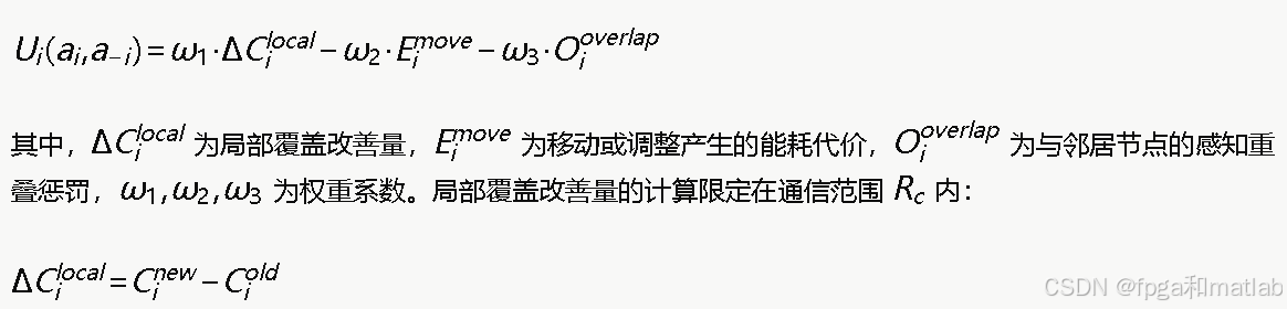AI Visual Insight: This figure shows the weighted composition of the utility function. The technical focus is to unify positive coverage reward and negative movement cost and overlap penalty under the same reward scale so that reinforcement learning can use this value directly for policy iteration.

% --- Game-theoretic weights ---
w_coverage  = 12.0;    % Coverage gain weight
w_move_cost = 0.015;   % Movement cost weight
w_range_cost = 0.008;  % Radius adjustment cost weight
w_overlap   = 0.003;   % Overlap penalty weight

% Reward example: larger coverage improvement is better,
% while movement and overlap should be minimized
reward = w_coverage * delta_cover ...      % Coverage improvement reward
       - w_move_cost * move_dist ...       % Movement consumption penalty
       - w_range_cost * abs(delta_range) ... % Radius change cost
       - w_overlap * overlap_area;         % Overlap region penalty

This code expresses an engineering-style implementation of the reward function. At its core, it creates a tunable tradeoff among coverage, energy consumption, and redundancy.

Q-Learning learns the optimal action in a dynamic environment

Each node maintains its own Q-table. The state is usually represented by the level of local coverage gap, while the action space contains discrete choices such as stay still, move up, down, left, or right, increase or decrease the sensing radius, or move toward the hole center.

Q-value updates are based on immediate reward and the maximum expected future return of the next state. As a result, even without an exact environment model, nodes can gradually learn strategies that are beneficial to themselves and to the network as a whole over many episodes.

AI Visual Insight: This figure presents the standard Q-Learning update equation. It highlights the four core variables: learning rate, discount factor, immediate reward, and the maximum Q-value of the next state. Together they represent the temporal-difference update mechanism of model-free reinforcement learning.

AI Visual Insight: This figure describes how local coverage gaps are mapped to discrete state indices. It shows how continuous coverage quality is compressed into a finite state space so that tabular Q-Learning can be implemented directly in MATLAB.

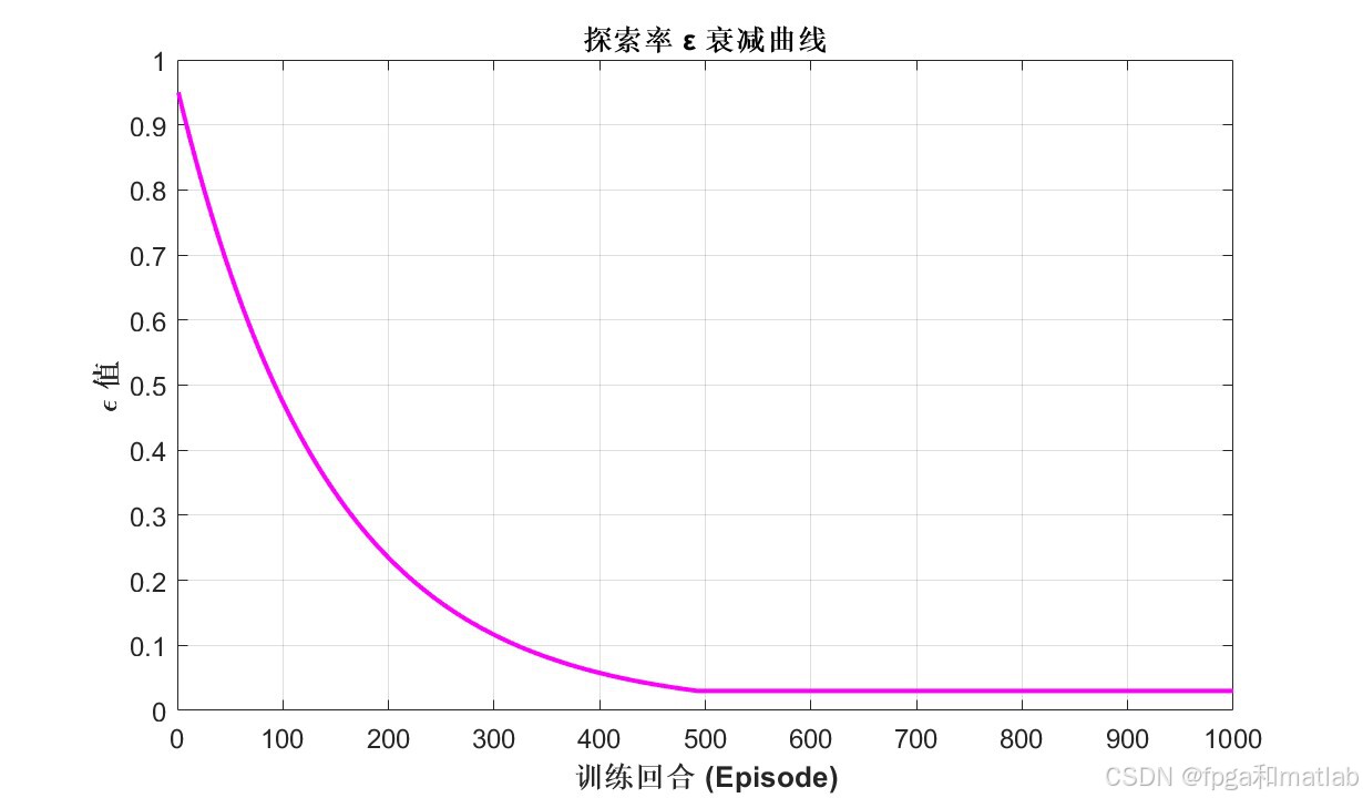
AI Visual Insight: This figure shows the exploration-rate decay formula in the ε-greedy strategy. Its technical role is to encourage random exploration in the early stage and gradually shift toward exploiting high-value learned actions later, balancing convergence speed and global optimum search.

% --- Q-learning parameters ---
num_episodes = 1000;   % Number of training episodes
max_steps = 20;        % Maximum steps per episode
alpha_lr = 0.025;      % Learning rate
gamma_df = 0.99;       % Discount factor
eps = 0.95;            % Initial exploration rate

% Q-value update
Q(s,a) = Q(s,a) + alpha_lr * ( ...
    reward + gamma_df * max(Q(s_next,:)) - Q(s,a)); % Update Q-table by temporal difference

eps = max(0.03, eps * 0.993);  % Gradually reduce exploration rate

This code implements the core iteration of tabular Q-Learning. It is also the key mechanism that moves the algorithm from random trial and error toward stable hole recovery.

The simulation results show that the method optimizes more than coverage alone

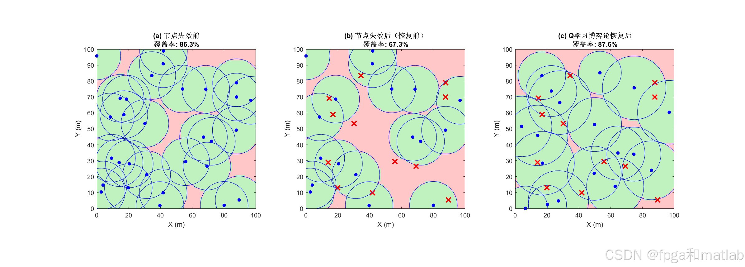
AI Visual Insight: This figure typically shows the initial node deployment or the coverage distribution after node failures. It helps reveal the hole regions created by failed nodes and the spatial distribution of surviving nodes.

AI Visual Insight: This figure reflects the node relocation or sensing-radius adjustment result after the algorithm runs. Technically, it can be used to compare hole reduction and cooperative migration trends before and after recovery.

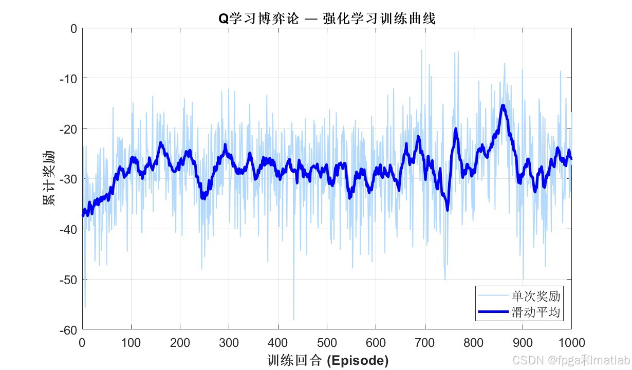
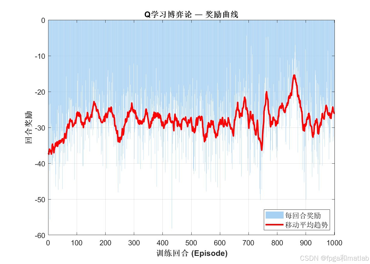
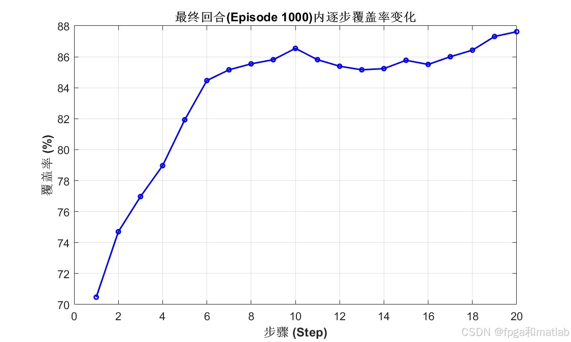
AI Visual Insight: This figure most likely presents coverage ratio, reward value, or convergence curves during training. It is used to verify whether Q-Learning steadily improves policy quality after multiple episodes.

AI Visual Insight: This figure may compare different strategies in terms of energy consumption, movement distance, or overlap ratio. It shows that the algorithm does not aim only at maximizing coverage, but at optimizing overall performance.

AI Visual Insight: This figure usually corresponds to the final recovery overview. It allows you to observe hole closure quality, node distribution balance, and whether the recovery strategy creates local crowding or misses boundary areas.

The source material makes three evaluation goals clear: whether holes shrink, whether coverage improves, and whether the recovery process converges. If you extend the experiments further, it is worth adding side-by-side comparisons with pure mobility methods, pure power-adjustment methods, and PSO-based approaches.

This approach fits distributed scenarios with limited resources and dynamic environments

It is especially suitable for area-based WSN applications such as disaster monitoring, agricultural sensing, and border inspection. In these scenarios, manual maintenance is infrequent, and local node failures are often random.

That said, the approach also has limitations. Tabular Q-Learning is sensitive to state dimensionality, and the Q-table grows rapidly as the network scale increases. For larger networks, you can introduce function approximation or multi-agent deep reinforcement learning.

FAQ

Q1: Why combine game theory with Q-Learning instead of using only one method?

A: Game theory constrains multi-node coordination so that local decisions stay aligned with the global objective as much as possible. Q-Learning learns action values through trial and error in an unknown and dynamic environment. Together, they provide both a theoretical convergence framework and environmental adaptability.

Q2: What are the most important tunable parameters in this MATLAB simulation?

A: Focus first on the learning rate alpha, discount factor gamma, epsilon decay, coverage gain weight, movement cost weight, and overlap penalty weight. These parameters directly control convergence speed, recovery aggressiveness, and the energy-performance balance.

Q3: What should be added first before applying this method to a real WSN system?

A: You should first add realistic packet loss behavior, a residual energy model, boundary obstacle constraints, and continuous action control. The discrete grid and discrete actions in the simulation are appropriate for validating the concept, but engineering deployment usually requires more refined physical modeling.

Core summary

This article reconstructs a hybrid coverage hole recovery approach for wireless sensor networks. It uses a potential game to unify node coordination and then applies Q-Learning to learn movement and sensing-radius adjustment strategies from local information, achieving a balance among coverage improvement, energy constraints, and overlap suppression.