This article builds an end-to-end solution for slope early warning: data calibration → stage identification → anomaly detection → stage-wise forecasting → warning thresholds. It addresses strong noise, missing values, abrupt changes, and multi-source coupled modeling. Keywords: slope early warning, change point detection, multi-source time series.
Technical Specifications Snapshot
| Parameter | Details |
|---|---|
| Application Domain | Slope hazard monitoring and early warning |
| Core Data | Displacement, rainfall, pore water pressure, microseismic activity, blasting variables |
| Modeling Languages | Python / MATLAB |
| Key Methods | Regression calibration, PELT/SG filtering, MICE, XGBoost, LSTM |
| Data Format | Time-series CSV/XLSX, 10-minute or irregular sampling |
| Stars | Not provided in the source content |
| Core Dependencies | pandas, numpy, scikit-learn, ruptures, xgboost, statsmodels |
This problem is fundamentally about designing a multi-source time-series early warning system
Problem C is not a standalone forecasting task. It is a typical engineering monitoring pipeline reconstruction problem. It requires you to connect sensor bias, non-stationary deformation, abnormal disturbances, missing data, and warning logic into one unified framework.
From the task structure, the five subproblems are tightly coupled. Problem 1 provides a trustworthy displacement baseline, Problem 2 defines stage labels, Problem 3 completes data governance, Problem 4 performs stage-wise prediction, and Problem 5 outputs actionable warning rules.
The recommended modeling backbone is as follows
pipeline = [
    "Sensor calibration",      # First, unify the displacement baseline
    "Stage identification",   # Then identify slow / accelerated / rapid stages
    "Denoising and imputation",# Clean multi-source monitoring variables
    "Stage-wise forecasting", # Train separate models for each stage
    "Threshold-based warning" # Finally, build a three-level yellow-orange-red warning system
]
This pipeline defines the most stable answer structure for the entire problem.
Problem 1 should be framed as a baseline-sensor-driven bias correction task
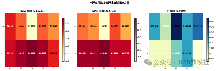
Dataset A comes from a fiber optic displacement meter, while Dataset B is the vibrating-wire reference. The goal is not a simple translation. You need to identify constant offset, linear drift, or nonlinear installation error, and control generalization error through cross-validation.
Start with aligned A/B time-series plots and residual plots. If the residuals grow approximately linearly, use linear regression. If the behavior differs across intervals, piecewise regression or spline fitting is more robust.
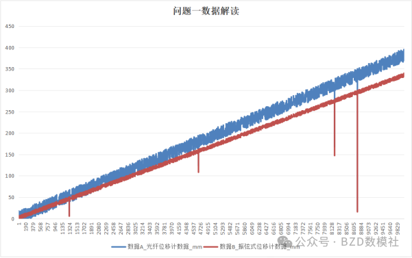 AI Visual Insight: The figure shows the overall trend alignment between two displacement series on the same time axis. A and B follow similar growth patterns, but a stable offset or slope difference is visible, which indicates that the calibration model should prioritize systematic error rather than random noise.
from sklearn.linear_model import LinearRegression

# Use A to predict B and build a calibration mapping
model = LinearRegression()
model.fit(A.reshape(-1, 1), B)  # Learn the mapping from fiber displacement to reference displacement
B_hat = model.predict(A.reshape(-1, 1))
This code maps the raw A series into the scale and trend space of the reference B series.
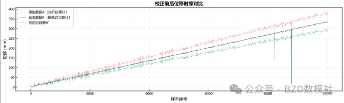 AI Visual Insight: The figure likely shows the post-calibration fit or residual trend. The key is whether the model error converges in both low-displacement and high-displacement ranges, which helps determine whether structural bias still remains.
 AI Visual Insight: This figure may compare results before and after calibration. If the two curves align at the major turning points, the model not only corrects mean bias but also preserves the true deformation dynamics.
Problem 2 requires combining change point detection with engineering criteria
Three-stage deformation identification cannot rely only on algorithm output. Real transition points must satisfy the condition that increased velocity persists after the change, while noise spikes usually fall back quickly after a sharp jump.
Therefore, apply median filtering or Savitzky-Golay smoothing first, then perform change point detection on the first-difference velocity series. PELT is suitable for locating structural breakpoints, but you must add duration constraints and posterior trend constraints.
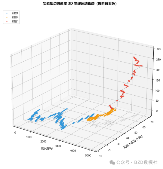
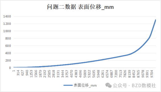 AI Visual Insight: The figure shows a stage transition in which the displacement curve changes from slow growth to steep increase. The core signal is a sustained slope increase near two turning points rather than a single-point spike, which is exactly what distinguishes real instability evolution from transient disturbance.
The criteria for true transition nodes should be stated explicitly in the paper
- The mean post-change velocity is significantly higher than that of the previous segment.
- The new velocity level persists for several windows without reverting.
- The slope of the cumulative displacement curve changes permanently.
- Acceleration remains with the same sign locally or is positive overall.
import ruptures as rpt

signal = velocity.values  # Perform change point detection on the velocity series, not raw displacement
bkps = rpt.Pelt(model="rbf").fit(signal).predict(pen=8)
This code automatically identifies structural changes in velocity and then filters valid transition points using engineering rules.
Problem 3 is essentially a data governance task for heterogeneous monitoring variables
The five variable groups have very different statistical properties, so you should not smooth them uniformly. Rainfall is sparse and pulse-like, so preserve raw peaks. Pore pressure and displacement are continuous and slowly varying, so SG filtering is appropriate. Microseismic activity is count-based and discrete, so a rolling median is more suitable.
Missing-value completion should also be layered. For short gaps, use cubic spline interpolation. For long gaps, combine cross-variable correlations through MICE or regression imputation. This preserves coupling information across variables rather than relying only on the local trend of a single series.
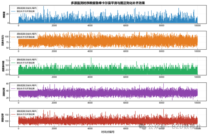 AI Visual Insight: The figure most likely shows the multivariate time-series distribution in the training set or a before/after denoising comparison. You can observe differences in fluctuation scale and anomaly spike density across variables, which supports differentiated denoising strategies.
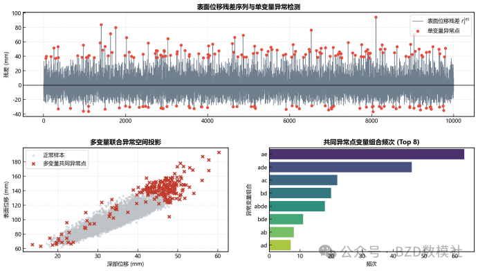 AI Visual Insight: The figure may show missing-value reconstruction or anomaly localization. If anomalies appear synchronously across multiple variables, they are more likely to indicate an engineering event or a real precursor to failure rather than a single-sensor fault.
Anomaly detection should include both univariate and joint anomaly identification
You can first use Hampel, IQR, or STL residuals for univariate detection, then count whether at least two variables are abnormal at the same timestamp. Joint anomalies carry more engineering meaning and are more suitable for downstream warning feature construction.
# Use a boolean matrix to count joint anomalies
joint_abnormal = (abnormal_matrix.sum(axis=1) >= 2)
joint_index = data.index[joint_abnormal]
This code extracts timestamps at which multiple variables become abnormal simultaneously.
Problem 4 should use stage-wise forecasting instead of a single global model
The transition nodes in the training set and experimental set are not identical, but the problem statement says that the stage-wise patterns are consistent. That means the modeling unit is not absolute time, but stage mechanism. The slow stage is closer to linear behavior, while the rapid stage is more nonlinear. A single model would dilute those patterns.
A practical strategy is as follows: use linear regression or ARIMA for Stage 1, random forest or XGBoost for Stage 2, and LSTM or gradient boosting trees for Stage 3. If blasting variables are almost entirely missing, set them to zero first and add a missing-indicator feature.
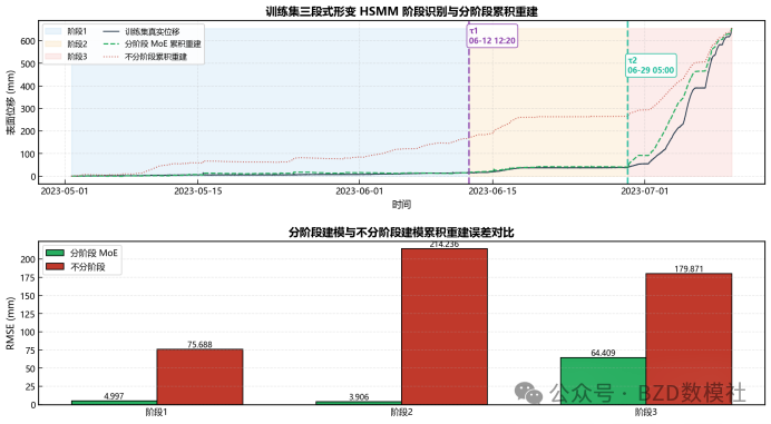 AI Visual Insight: The figure reflects stage-wise modeling results or differences in feature impact. The main point is that fitted slopes, residual distributions, and responses to external disturbances differ significantly across stages.
 AI Visual Insight: This figure may show the alignment between model predictions and actual displacement. If the model still tracks sharp increases in the accelerated and rapid stages, then the stage-wise approach outperforms a global average model.
 AI Visual Insight: The figure should represent the prediction curve on the experimental set. The technical focus is to invoke models segment by segment according to the given stage labels and then stitch the outputs together while keeping transitions continuous and stable.
The implementation template for stage-wise forecasting can be organized like this
for stage in [1, 2, 3]:
    sub = train[train["stage"] == stage]
    model = train_stage_model(sub)  # Train a dedicated predictor for each stage
    pred[exp["stage"] == stage] = model.predict(exp_features_of_stage(stage))
This code trains by stage and performs inference by stage, which matches the mechanism defined in the problem.
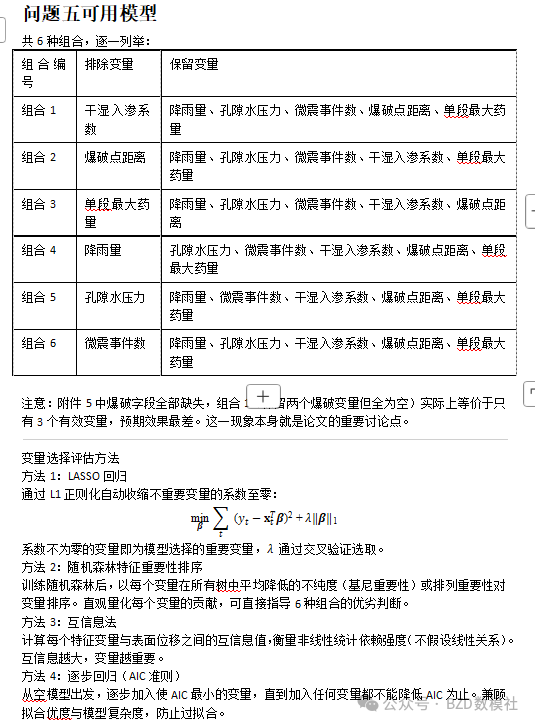
Problem 5 ultimately outputs the optimal variable combination and executable warning thresholds
For variable selection, use a strategy of performance first with interpretability constraints. Exhaustively evaluate 6-choose-5 combinations or apply recursive feature elimination, then compare them using RMSE, MAE, and R². Since blasting-related variables are missing across large portions of the appendix data, they will likely be identified as low-contribution features.
For warning indicators, use displacement velocity as the unified metric and set thresholds by stage. In the slow stage, thresholds should be lower and prioritize sensitivity. In the rapid stage, thresholds should be higher and prioritize failure confirmation. You can define three alert levels using quantiles, the Fukuzono inverse-velocity concept, or stage-wise mean ± standard deviation.
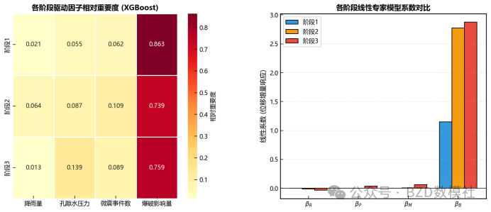
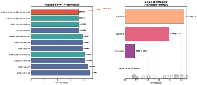 AI Visual Insight: The figure may correspond to variable combinations or feature-importance comparisons, making it easy to see ranking differences in how rainfall, pore pressure, microseismic activity, and infiltration coefficient contribute to displacement prediction.
 AI Visual Insight: The figure shows a warning-threshold partitioning method or velocity distribution boundaries. Technically, it is used to convert a continuous risk metric into discrete alert levels.
 AI Visual Insight: The figure may illustrate response intervals or sample positions under different warning levels, which helps verify whether the thresholds are both discriminative and stable.
 AI Visual Insight: This figure should show the final warning mechanism. The key is the closed-loop flow from monitoring data input to velocity calculation, stage identification, and yellow-orange-red alert output.
The key to a high-scoring solution is a unified narrative loop
The best answer does not treat each subproblem as an isolated model. Instead, it emphasizes the progression from a trustworthy displacement baseline to reliable stage labels, clean multi-source features, stage-wise forecasting, and velocity-based warning. This makes the paper read like an engineering system rather than a collection of disconnected solutions.
For a stronger implementation-oriented write-up, add four result types: a calibration error table, a change point index table, an anomaly count table, and an experimental-set prediction table. These directly correspond to the main scoring points of the problem.
FAQ
Q: Why should Problem 2 not perform change point detection directly on raw displacement?
A: Raw displacement is usually monotonically cumulative, so the long-term trend can mask local stage changes. Running change point detection on smoothed velocity or increment series makes it easier to identify structural transitions from slow to accelerated deformation.
Q: Why can Problem 3 not use a single linear interpolation strategy for all missing values?
A: Because rainfall, microseismic activity, pore pressure, and displacement follow different statistical mechanisms. A uniform linear interpolation approach would flatten pulse events and cross-variable coupling, which would distort downstream anomaly detection and forecasting models.
Q: How can the warning thresholds in Problem 5 be justified?
A: You can justify them from three perspectives: differences in stage-wise velocity distributions, hit rate on historical anomaly points, and the false-positive/false-negative tradeoff under different thresholds. If you also incorporate inverse-velocity critical trends, the engineering argument becomes even more convincing.
Core Summary: This article reconstructs the May Day Mathematical Modeling C Problem as a directly implementable technical solution. It covers fiber optic displacement meter calibration, three-stage deformation identification, multi-source monitoring data denoising and imputation, stage-wise displacement forecasting, optimal variable combination selection, and warning-threshold design. It is suitable for paper writing, code implementation, and defense preparation.