This article focuses on PyTorch’s core capabilities for vision detection. It explains tensor computation, automatic differentiation, CNNs, YOLO, and industrial defect detection workflows, addressing three common pain points: fragmented theory, difficult implementation, and broken engineering pipelines. Keywords: PyTorch, object detection, defect detection.
Technical specification snapshot
| Parameter | Description |
|---|---|
| Core languages | Python, C++, CUDA |
| Core framework | PyTorch |
| Task types | Image classification, object detection, defect detection |
| Representative protocols/paradigms | Autograd, DDP, one-stage detection |
| Typical models | CNN, YOLO, ResNet |
| Core dependencies | torch, torch.nn, torch.distributed, PyTorch Lightning |
| Data characteristics | High-dimensional tensors, bounding boxes, class labels |
| GitHub stars | Original data not provided |
PyTorch provides an efficient foundation for vision detection engineering
PyTorch is best understood as “NumPy with GPU support plus an automatic differentiation system.” It solves two classic problems in numerical computing: CPU-only execution and the difficulty of manually deriving gradients for deep networks. That is why it has become a mainstream training framework for vision tasks.
In vision workloads, images are represented as tensors. Compared with NumPy arrays, tensors can move seamlessly to GPUs and participate in automatic differentiation. This means the same forward logic can support both rapid prototyping and full model training.
Tensor operations are the basic entry point for visual modeling
import torch

# Create a 2D tensor to simulate a small feature map
x = torch.tensor([[1., 2., 3.],
                  [4., 5., 6.],
                  [7., 8., 9.]])

# Power operation: commonly used for numerical transformation
print(x.pow(2.0))

# Sum by column: can be understood as aggregating features along columns
print(x.sum(dim=0))

# Sum by row and then take the reciprocal: common in normalization pre-processing
temp = x.sum(dim=1).pow(-1.0)

# Generate a diagonal matrix: used for weight scaling or mask construction
print(temp.diag_embed())
This code demonstrates basic tensor operators. They are the low-level building blocks behind convolution, normalization, and loss computation.
Automatic differentiation shifts training from manual calculus to computation graph execution
The key to neural network training is backpropagation. PyTorch Autograd records the chain of operations during the forward pass. Developers only need to define the computation, and gradients are generated automatically through .backward().
This changes model design from “derive complicated gradients first” to “express computation logic first.” It significantly lowers experimentation costs and makes debugging feel much closer to standard Python programming.
Autograd reduces the complexity of handwritten gradients
import torch

# Create a scalar that requires gradients
x = torch.tensor(2.0, requires_grad=True)

# Forward computation: y = x^2
y = x ** 2

# Backpropagation: automatically compute dy/dx
y.backward()

# Print the gradient; the theoretical value is 2x = 4
print(x.grad)
This example shows that PyTorch automatically tracks the computation graph and propagates gradients.
Dynamic computation graphs make model debugging and complex architectures more direct
PyTorch builds its dynamic computation graph at runtime instead of requiring a define-then-compile workflow like early static-graph frameworks. This is especially friendly for research-oriented development, because loops, conditionals, and intermediate print statements fit naturally into the code.
In vision detection, this capability is ideal for quickly testing different Backbone, Neck, and Head combinations. It also makes it easier to diagnose gradient anomalies, shape mismatches, and non-converging losses.
Multi-GPU training is a critical path for scaling vision models
DataParallel is commonly used for multi-GPU training on a single machine, but it overloads the primary GPU. DistributedDataParallel is generally the better choice because each GPU computes independently and synchronizes gradients, which improves throughput and stability.
import torch
import torch.nn as nn
from torch.nn.parallel import DistributedDataParallel as DDP

# Initialize the distributed communication environment
torch.distributed.init_process_group(backend="nccl")

model = nn.Linear(128, 10).cuda()

# Wrap the model with DDP and bind it to the GPU for the current process
model = DDP(model, device_ids=[0])
This snippet shows the minimum DDP setup, which is the standard approach for large-scale vision training.
If you want to reduce engineering boilerplate, PyTorch Lightning can take over the training loop quickly through accelerator="gpu" and strategy="ddp".
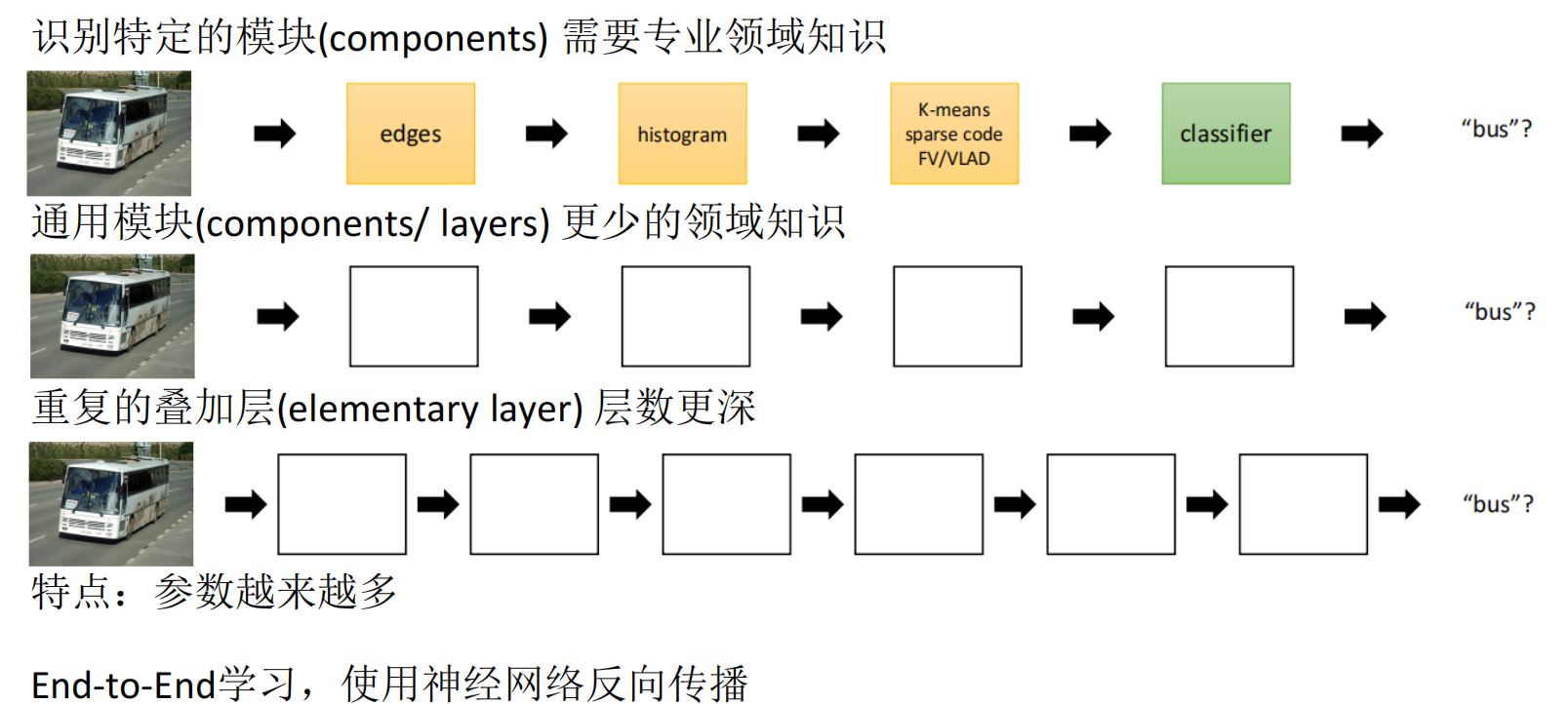
Image recognition is fundamentally a hierarchical abstraction from pixels to semantics
A typical vision recognition pipeline includes data acquisition, preprocessing, feature extraction, classification, and output. Traditional methods rely more on manually designed features, while deep learning learns high-dimensional representations directly from data.
The rise of ImageNet accelerated the modern computer vision boom. After AlexNet, architectures such as VGG, GoogLeNet, ResNet, and DenseNet continued to push accuracy higher and established CNNs as the dominant backbone for recognition and detection tasks.
Convolution and activation functions form the basic operators of vision networks
import torch
import torch.nn.functional as F

# Simulate an input image: 1 image, 3 channels, 64x64
x = torch.randn(1, 3, 64, 64)

# Define convolution kernels: output 16 feature channels
weight = torch.randn(16, 3, 3, 3)

# Run 2D convolution followed by ReLU activation
y = F.conv2d(x, weight, stride=1, padding=1)
y = F.relu(y)

# Max pooling: reduce spatial size while preserving strong responses
y = F.max_pool2d(y, kernel_size=2)
print(y.shape)
This code maps directly to the typical local feature extraction flow in CNNs: convolution, activation, and pooling.
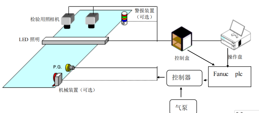
Industrial defect detection is not purely an algorithm problem but a hardware-software system
In industrial environments, traditional vision solutions rely on measurable rules such as color, area, roundness, length, and edges. Their strengths are interpretability and fast deployment. Their weakness is limited generalization: once lighting, material, or production batches change, the rules may fail.
Deep learning-based detection can learn complex patterns from samples and is usually more robust to illumination variation, curved-surface reflections, and texture disturbances. However, the cost shifts to data collection, annotation, and training resources. When data is limited, transfer learning is often more practical than training from scratch.
 AI Visual Insight: This image compares traditional vision with deep learning-based visual inspection. It highlights the difference between rule-driven and data-driven paradigms in adaptability, feature extraction, and scene complexity, making it useful for explaining why industrial inspection often needs to migrate from OpenCV rule systems to CNN models.
Defect detection solution design must first constrain the data and on-site conditions
Before designing a solution, answer four questions: Are there enough defect samples? How do humans distinguish defects? Is there similar public data available? Can on-site hardware be adjusted? In many cases, poor model accuracy is not caused by the network itself but by image acquisition quality.
Industrial cameras are usually better than smartphones not because they always have more pixels, but because they often have larger sensors and better light intake, making them better suited for high-speed and low-light environments. Monochrome cameras also often outperform color cameras in edge detection and subtle defect inspection.
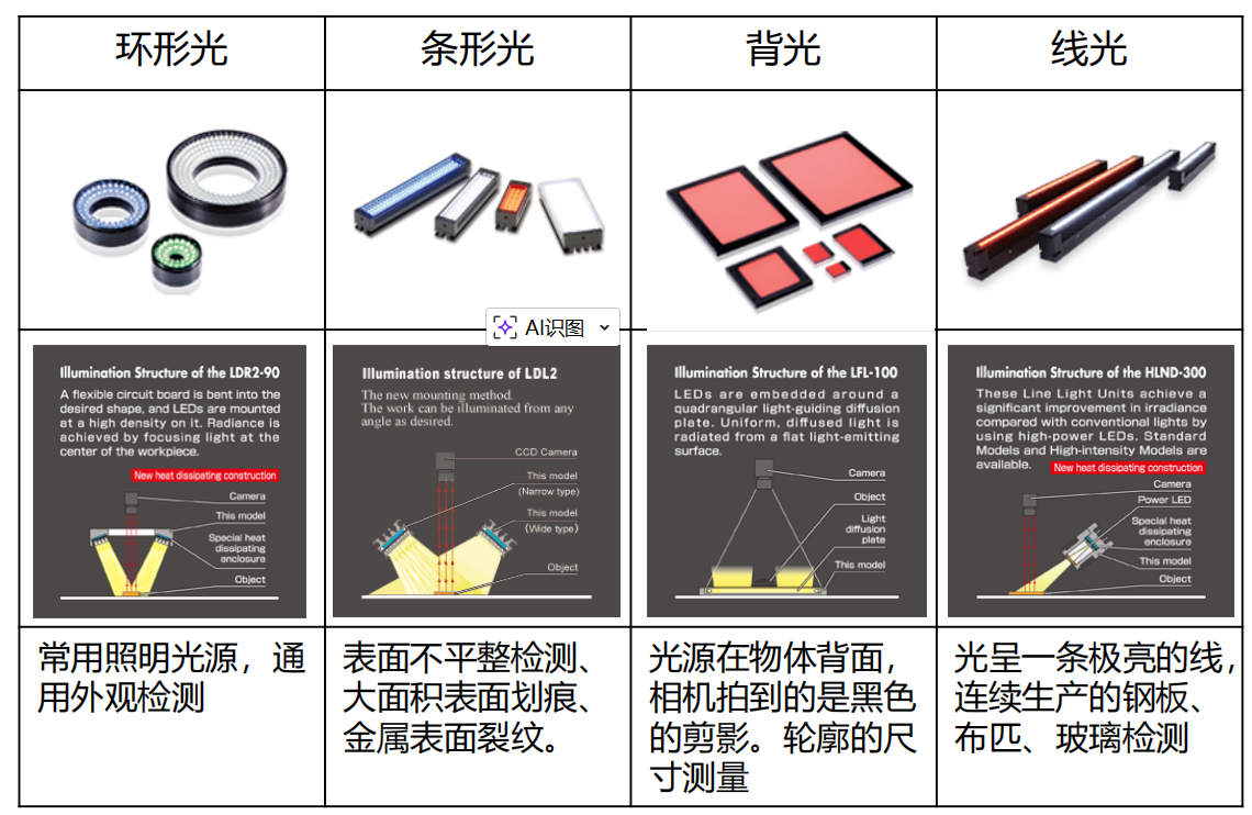 AI Visual Insight: This image shows the physical appearance of different industrial lighting forms and illumination devices. It helps explain how ring lights, bar lights, and similar setups differ when selected for surface defects, edge enhancement, and reflection control.
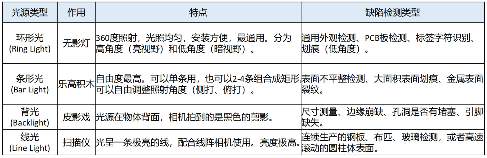 AI Visual Insight: This image further supplements multiple light source structures and installation methods. It shows that image quality in machine vision depends on the combination of light source type, installation angle, and target material—not on algorithm tuning alone.
 AI Visual Insight: This image illustrates how direct light, reflected light, and diffuse light affect imaging results. The core takeaway is that the same defect can appear with completely different contrast under different incident angles, so lighting is a major upstream variable in defect detection accuracy.
CNNs extract hierarchical features through local receptive fields and weight sharing
The core ideas behind CNNs are local connectivity and parameter sharing. A convolution kernel slides across the image and reuses the same weights at different positions, which makes it efficient at extracting local patterns such as edges, textures, and shapes.
As the network depth increases, features evolve from low-level edges to textures, parts, and complete objects. This is why CNNs work reliably in image classification, face recognition, and defect localization.
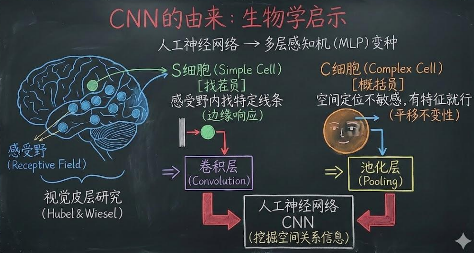 AI Visual Insight: This image shows how convolutional networks evolved under the influence of biological vision research. It emphasizes the origins of local receptive fields, hierarchical responses, and spatial structure modeling, helping explain why CNNs are well suited for two-dimensional image signals.
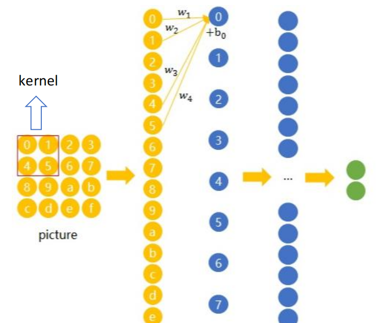 AI Visual Insight: This image visualizes how a convolution kernel slides over an input feature map. It highlights weight sharing, local region mapping, and the output feature generation process, making it an intuitive explanation of Conv2d.
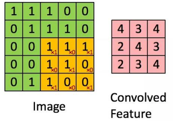 AI Visual Insight: This image shows how feature maps become more abstract across multiple convolution layers. It reflects the fact that training continuously optimizes convolution kernel weights so the network can move from low-level textures to high-level semantic responses.
YOLO turns object detection into a single forward regression problem
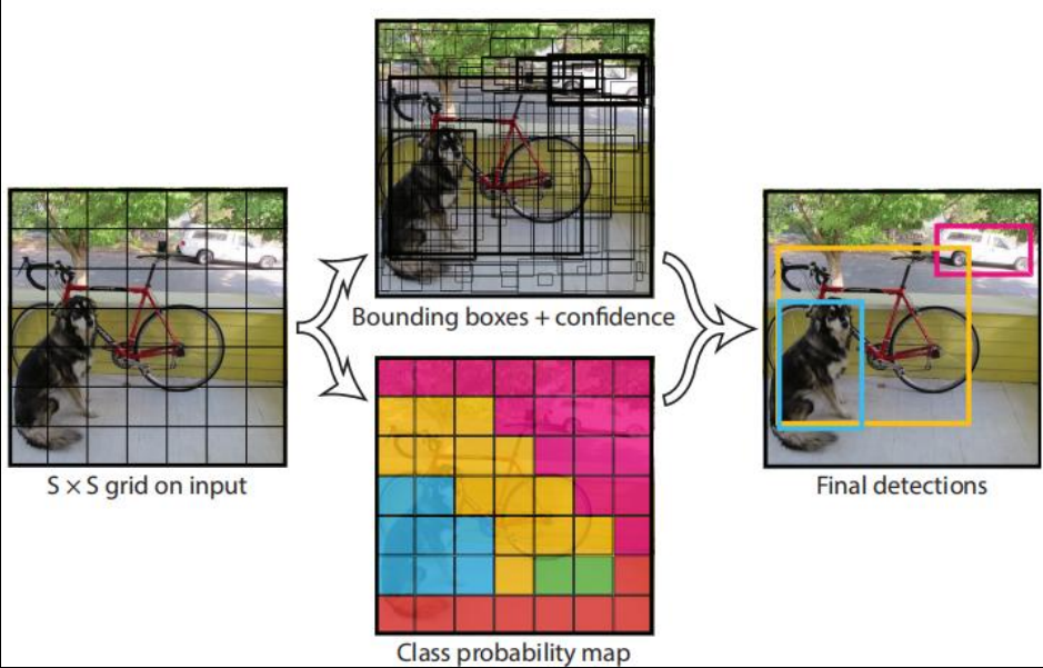
YOLO differs from traditional two-stage detectors because it directly regresses object locations and classes from the entire image instead of generating region proposals first. As a result, it is fast, structurally unified, and well suited for real-time detection scenarios.
Its core mechanism divides the image into an S×S grid. Each grid cell predicts multiple bounding boxes and confidence scores, along with class probabilities. If the center of an object falls into a grid cell, that cell is responsible for predicting the object.
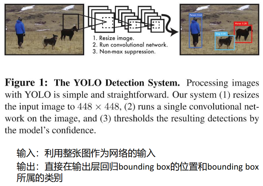 AI Visual Insight: This image shows how YOLO maps a full input image into a unified detection output. It emphasizes the one-stage design principle of producing class and localization results in a single forward pass.
YOLOv1 defined the basic paradigm for real-time detection
If S=7, B=2, and the number of classes C=20, then the output tensor shape is 7×7×30. Each grid cell contains class probabilities, bounding box coordinates, and confidence information.
S, B, C = 7, 2, 20

# Compute the last dimension of the YOLOv1 output tensor for one image
output_dim = B * 5 + C  # 2 boxes * 5 parameters + 20 classes
print(S * S * output_dim)

# The output is 1470, which equals 7*7*30
This code corresponds to the classic YOLOv1 output dimension calculation.
 AI Visual Insight: This image clearly demonstrates how the image is divided into regular grids and how each grid predicts multiple candidate boxes. It uses border thickness or intensity to express confidence differences, making it a key illustration for understanding YOLO grid responsibility assignment.
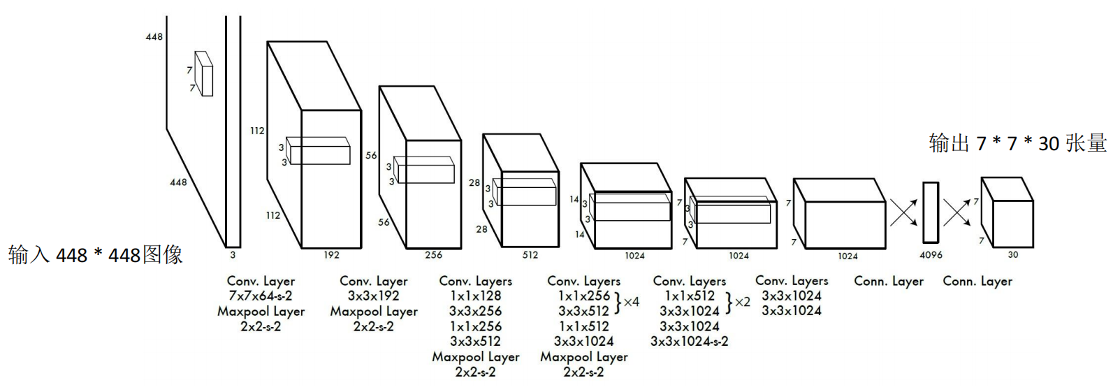 AI Visual Insight: This image shows the YOLOv1 network architecture, which typically includes convolutional feature extraction layers and fully connected prediction layers. It reflects the early engineering trade-offs behind YOLO’s unified detection head.
Non-maximum suppression keeps the best result from redundant candidate boxes
The same object is often detected by multiple boxes at once. The purpose of NMS is to sort candidates by confidence and then remove boxes that overlap too much with the current best box, producing a cleaner final detection result.
IoU is the core metric behind NMS. It represents the intersection-over-union ratio between a predicted box and a ground-truth box, or between two candidate boxes. The higher the IoU, the greater the overlap.
def nms_step(box_scores, iou_threshold=0.5):
    # box_scores: [(box, score), ...], sorted from high to low by score
    selected = []
    for box, score in box_scores:
        keep = True
        for chosen_box, _ in selected:
            iou = compute_iou(box, chosen_box)  # Compute IoU between two boxes
            if iou > iou_threshold:
                keep = False  # Overlap is too large; suppress the current candidate box
                break
        if keep:
            selected.append((box, score))
    return selected
This pseudocode summarizes the core NMS workflow: sort, compare IoU, and keep locally optimal boxes.
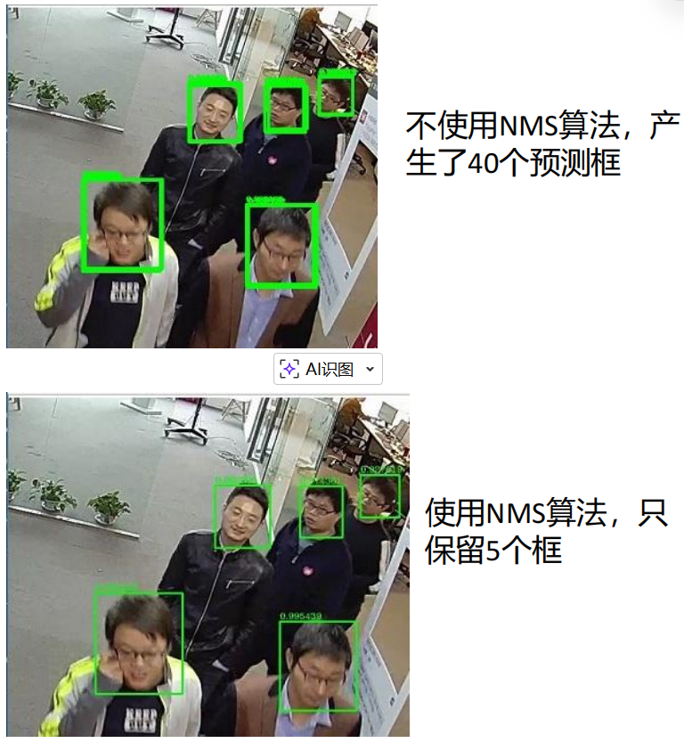 AI Visual Insight: This image shows multiple candidate boxes overlapping around the same object. It explains why NMS is necessary: without it, the model would output multiple high-confidence boxes for the same object, which reduces practical usability.
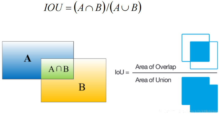 AI Visual Insight: This image explains the geometric meaning of IoU as the ratio of intersection area to union area. It is the foundational metric for measuring box overlap, assigning positive and negative samples, and executing NMS.
The knowledge path from PyTorch to YOLO covers most vision detection scenarios
From a learning perspective, the most effective order is to first master tensors, Autograd, convolution, and pooling; then understand how CNNs extract features; and finally move to YOLO, NMS, and engineering deployment. This creates a closed loop between framework capabilities and detection tasks.
From an industrial delivery perspective, the deciding factor is usually not the model name alone, but the combined optimization of data quality, lighting design, camera selection, labeling strategy, transfer learning, and training infrastructure.
FAQ
1. Why do many vision tasks choose PyTorch first?
Because it combines dynamic graph debugging, mature automatic differentiation, strong GPU support, and a rich computer vision ecosystem. It is ideal for moving quickly from research prototypes to engineering-scale training.
2. If model accuracy is low in industrial defect detection, is the algorithm always the problem?
Not necessarily. On-site lighting, lenses, cameras, exposure, and installation angles all strongly affect input quality. In many scenarios, improving imaging first delivers more value than tuning the model first.
3. How should I choose between YOLO and the traditional R-CNN family?
If you prioritize real-time performance, deployment efficiency, and a unified architecture, YOLO is usually the better fit. If you care more about absolute accuracy and can afford higher inference cost, two-stage methods often have an advantage.
Structured summary
This article systematically reconstructs the core knowledge behind PyTorch and vision detection. It covers tensor computation, automatic differentiation, dynamic graphs, CNNs, YOLO, NMS, and industrial defect detection design, while also adding engineering considerations such as cameras, lighting, and transfer learning. The goal is to help developers build a complete understanding from framework fundamentals to real-world deployment.