Q-Learning for 3D UAV Path Planning: Matlab Modeling and Optimization in Complex Urban Environments - Devuly | Smart Analytics for Developers & Projects

This article explains a 3D UAV path planning method designed for dense and complex urban environments. At its core, Q-learning learns an optimal policy for obstacle avoidance and goal reaching in a 3D grid space, addressing the heavy computation and weak adaptability of traditional global search in high-dimensional environments. Keywords: UAV path planning, Q-learning, Matlab.

Table of Contents

Technical Specifications Snapshot

Parameter	Details
Research Topic	3D UAV Path Planning
Core Algorithm	Q-learning
Implementation Language	Matlab
Environment Model	3D Grid Map
Learning Rate α	0.1
Discount Factor γ	0.9
Exploration Strategy	ε-greedy
ε Range	Decreases from 0.5 to 0.01
Maximum Iterations	50000
Reference Performance	85%+ success rate, about 30% shorter paths
License	Original source declares CC 4.0 BY-SA
Star Count	Not provided in the source material
Core Dependencies	Matlab matrix operations, 3D grid modeling, reinforcement learning logic

This research addresses low-altitude flight challenges in complex urban environments

The challenge of urban UAV path planning is not simply to “find a path,” but to continuously find a safe, executable, and low-cost path within constrained 3D space. Buildings, signal towers, and altitude restrictions all increase search complexity.

Traditional A* and Dijkstra perform reliably in static, low-dimensional spaces. However, once they move into dense 3D obstacle environments, the search space expands rapidly. The value of Q-learning is that it does not require an explicit environment model and can gradually learn a policy through interaction feedback.

The core Q-learning update rule maps directly to flight decisions

Q(s,a) = Q(s,a) + alpha * (r + gamma * max(Q(s_next,:)) - Q(s,a)); % Update the current action value using the temporal-difference error

This formula determines how the UAV merges “current reward” and “future optimal expectation” into the same Q-table.

3D grid modeling is the foundation for practical implementation

This approach uses a 3D grid map to represent urban space. Each grid point corresponds to a state, represented by coordinates (x, y, z), while also indicating whether it is an obstacle, whether it is out of bounds, and its relative position to the goal.

The state space can include more than position. It can also incorporate local environmental perception, such as neighborhood obstacle density, the direction of the nearest obstacle, or the target bearing. This reduces the perception blind spots of relying on “coordinates only.”

The action set must balance expressiveness and training cost

actions = [1 0 0; -1 0 0; 0 1 0; 0 -1 0; 0 0 1; 0 0 -1]; % Six basic actions for forward, backward, left, right, up, and down movement

This action design is simple and stable, making it suitable for tabular Q-learning. If diagonal actions are added, the path becomes more flexible, but the action space also grows accordingly.

The reward function determines whether a path is merely feasible or actually efficient

The reward function usually considers goal reaching, collision penalties, distance change, and flight cost at the same time. Reaching the goal gives a large positive reward, collisions incur a strong negative penalty, moving closer to the goal gives positive feedback, and each movement step adds a small cost.

This design essentially balances four goals: reachability, safety, convergence speed, and path length. If rewards are too sparse, learning slows down. If penalties are too strong, the agent may fall into overly conservative behavior.

if hit_obstacle
    r = -100; % Apply a strong penalty when colliding with an obstacle
elseif reach_goal
    r = 100;  % Give a high reward when reaching the goal
else
    r = dist_old - dist_new - 0.1; % Reward movement toward the goal and add a step cost
end

This logic unifies “obstacle avoidance first, goal seeking, and reduced detours” into a single-step feedback function.

The training process requires a dynamic balance between exploration and exploitation

During the early stage of training, the algorithm uses a larger ε so the UAV tries more unknown actions. As training progresses, ε is gradually reduced, shifting the policy from random exploration toward exploiting learned knowledge. This is one of the key conditions for Q-learning convergence.

The full workflow can be summarized as follows: initialize the Q-table, start from the initial state, choose actions with ε-greedy selection, receive rewards and the new state, update Q-values, repeat until the termination condition is met, and finally replay the optimal path from the Q-table.

A simplified Matlab training framework looks like this

for episode = 1:maxEpisode
    s = startState; % Restart from the initial state in each episode
    while ~isTerminal(s)
        a = chooseAction(Q, s, epsilon); % Select an action using the ε-greedy policy
        [s_next, r] = stepEnv(s, a, map); % Interact with the environment and return the next state and reward
        Q(s,a) = Q(s,a) + alpha * (r + gamma * max(Q(s_next,:)) - Q(s,a)); % Update the Q-table
        s = s_next; % Move to the next state
    end
    epsilon = max(0.01, epsilon * 0.995); % Gradually reduce the exploration rate
end

This framework fully covers the main Q-learning loop for path planning.

Experimental results show that the method is practical in complex environments

The original material uses the typical parameters α=0.1, γ=0.9, ε decreasing from 0.5 to 0.01, and a maximum of 50000 training iterations. Across multiple simulations, the algorithm achieves an average success rate above 85%.

Compared with random paths, the trained planner shortens path length by about 30% on average. This shows that Q-learning does not just find feasible routes, but gradually approaches lower-cost paths.

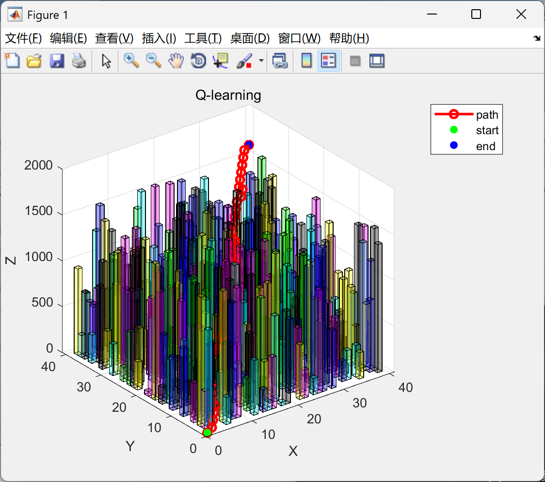AI Visual Insight: The image shows the flight space and obstacle distribution in a 3D urban scene. It is typically used to inspect the spatial relationship among the start point, end point, building volumes, and planned trajectory, helping verify whether the grid model correctly captures vertical constraints.

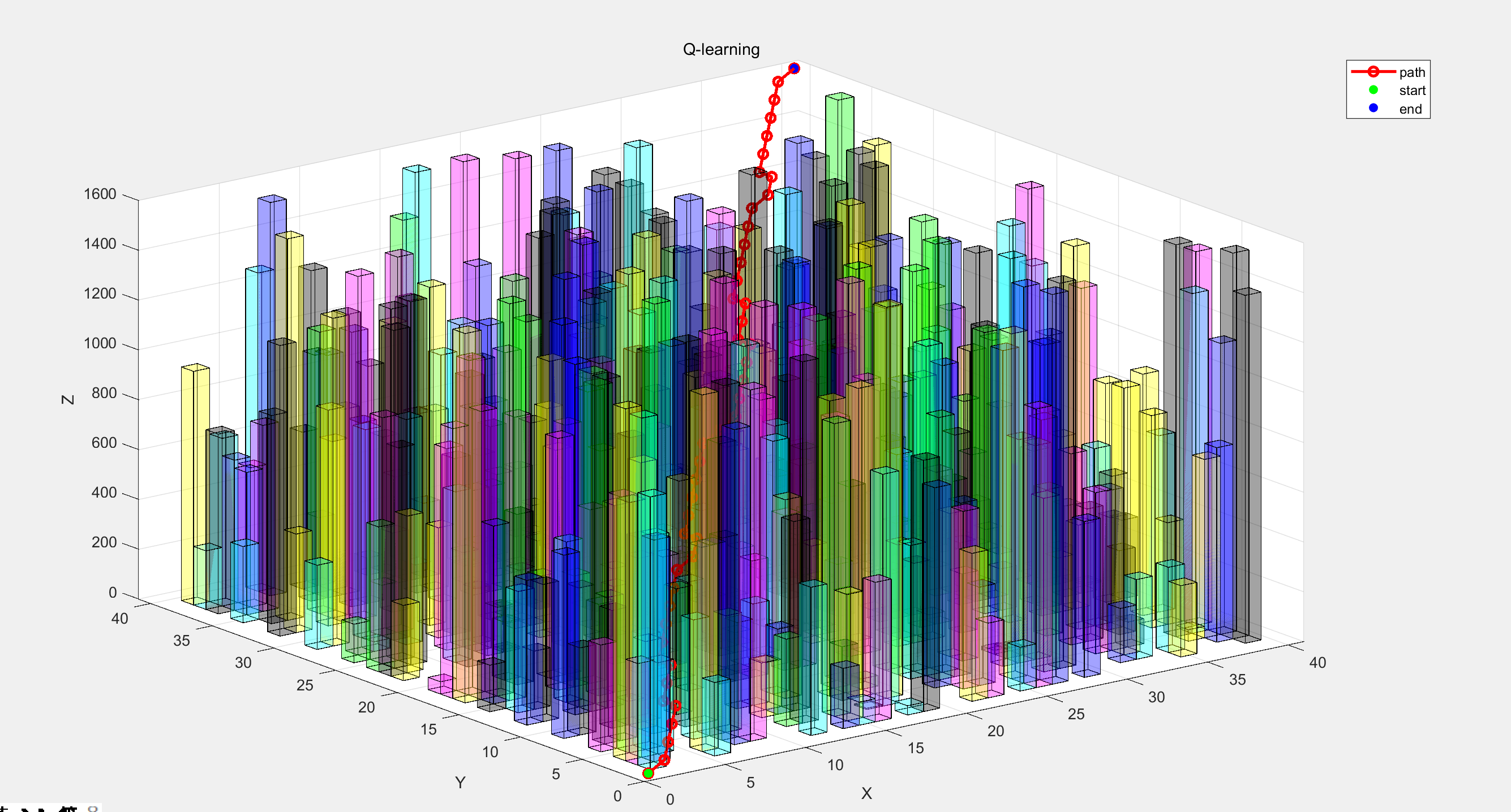AI Visual Insight: The image most likely presents the 3D flight trajectory during or after training. Key observations include whether the trajectory clearly detours around obstacles, whether it flies close to obstacle boundaries, and whether the path shows smooth and continuous spatial turning behavior.

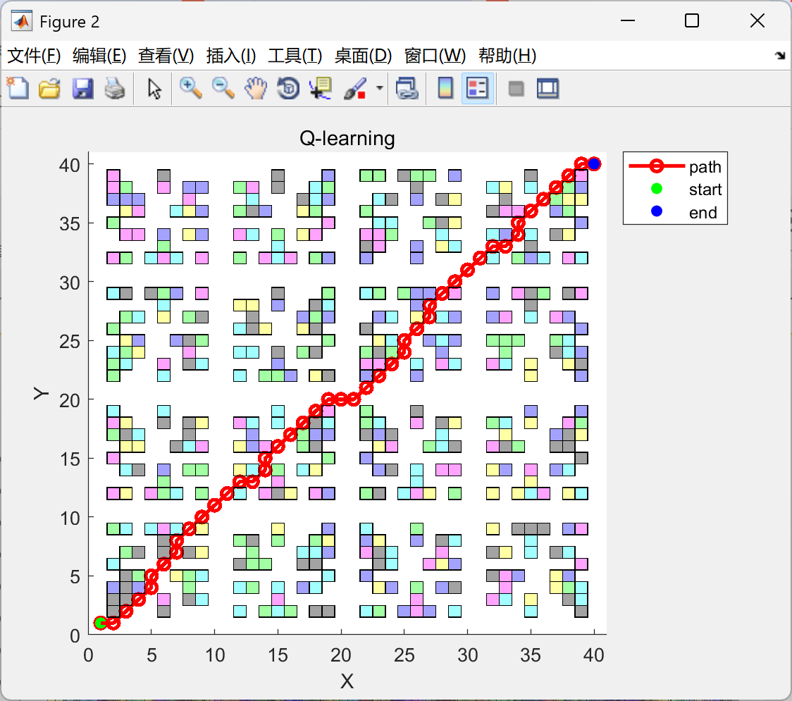AI Visual Insight: The image may reflect performance changes during algorithm convergence, such as cumulative reward, success rate, or path length across training episodes. It can help determine whether Q-learning converges stably and whether the convergence speed meets simulation requirements.

This method offers adaptive behavior rather than absolute optimality compared with traditional algorithms

A* can more easily produce a deterministic global path in known environments, but in complex 3D urban scenes, its search cost increases significantly with spatial dimensionality and obstacle density. Q-learning, by contrast, achieves online adaptability through experience-based learning.

However, Q-learning also has clear limitations: when the state space grows, the Q-table explodes; when training episodes are insufficient, path quality becomes unstable; and when facing dynamic obstacles, the standard tabular method has limited responsiveness.

Three common improvement directions deserve priority attention

Q_init = - heuristicDistToGoal(states); % Initialize Q-values with heuristic distance to reduce blind exploration

This type of initialization gives the agent an initial bias that “moving toward the goal is more valuable” from the start.

The other two effective directions are experience replay and hybrid optimization. The former improves stability by breaking sample correlation, while the latter can combine global optimization mechanisms such as Artificial Bee Colony to improve subgoal selection and reduce the probability of falling into local optima.

Three extension capabilities deserve priority in real-world engineering deployment

First, dynamic obstacle handling. Real urban low-altitude airspace includes moving targets such as vehicles, bird flocks, and UAV swarms. A static Q-table therefore requires either a time dimension or a shift toward deep reinforcement learning.

Second, large-scale scenario compression. You can reduce dimensional pressure with state aggregation, function approximation, or hierarchical planning.

Third, multi-UAV coordination. Single-agent optimality does not equal group optimality, and coordination constraints significantly change both reward design and state representation.

FAQ

Q1: Why choose Q-learning instead of A* in a 3D urban environment?

A1: Because Q-learning does not rely on an explicit environment model, it is well suited for learning policies in obstacle-dense scenarios with complex feedback and continuous trial-and-error. A* is better suited for deterministic search on static and known maps.

Q2: What is the biggest bottleneck when implementing this type of algorithm in Matlab?

A2: The main bottleneck is the rapid growth of Q-table storage and update cost caused by a large state space. The finer the 3D grid, the greater the training time and memory pressure, so implementations usually need to balance resolution and efficiency.

Q3: If I want to improve performance further, what should I optimize first?

A3: Start with the reward function and state representation, then move on to Q-value initialization, experience replay, and hybrid optimization. Many issues related to slow convergence or poor paths fundamentally come from unreasonable state and reward design.

Reference notes

This article reconstructs the method based on the provided original Markdown content. It preserves the research topic, key parameters, experimental conclusions, and Matlab implementation focus, while removing page noise, ads, and irrelevant navigation content.

AI Readability Summary: This article reconstructs a Q-learning-based 3D UAV path planning method, focusing on grid modeling, state-action design, reward functions, and Matlab implementation for dense urban environments. It also analyzes experimental results, convergence behavior, and the relative strengths and weaknesses of the approach compared with A*.