This article presents a 3D UAV path planning approach for complex mountainous environments, distilled into spherical-coordinate parameterization, 3D terrain and threat modeling, four-term collaborative cost optimization, and a unified comparison framework for multiple intelligent optimization algorithms. The core challenges are slow high-dimensional search, unsmooth trajectories, and the difficulty of unifying obstacle-avoidance constraints. Keywords: UAV path planning, intelligent optimization algorithms, MATLAB.
Technical Specifications at a Glance
| Parameter | Description |
|---|---|
| Implementation Language | MATLAB |
| Planning Space | 3D mountainous terrain |
| Path Representation | Piecewise chained parameterization in spherical coordinates |
| Constraint Types | Terrain, threat, altitude, smoothness |
| Compared Algorithms | PSO, GWO, WOA, HHO, DBO, SSA |
| Threat Modeling | Cylindrical no-fly / hazardous zones |
| Visualization Output | 3D view, top view, side view, convergence curves |
| Data Source | The original document does not provide a repository link or star count |
| Core Dependencies | MATLAB plotting, mesh, cylinder, lighting, colormap |
This Method Provides a Systematic Solution to the Core Bottlenecks of Mountain Flight
Mountain UAV path planning is not a simple shortest-path problem. It is a high-dimensional, non-convex, strongly constrained optimization problem. Rugged terrain, dense threat zones, and narrow flyable corridors simultaneously increase search complexity and the risk of generating infeasible trajectories.
The main value of the original approach is that it does not focus on a single algorithm in isolation. Instead, it first establishes a unified model and then performs a cross-algorithm comparison. This structure is better suited for engineering reproduction and also makes it easier for AI retrieval systems to extract key information.
Spherical-coordinate parameterization significantly reduces optimization dimensionality
Conventional methods often optimize a sequence of 3D waypoints directly, which causes the number of variables to grow linearly with path length. This approach instead uses step length, elevation angle, and azimuth angle to describe each path segment, transforming a high-dimensional discrete waypoint problem into a lower-dimensional continuous parameter problem.
This design delivers three direct benefits: fewer variables, more natural constraint handling, and trajectories that better match aircraft motion characteristics. In unified multi-algorithm testing, lower-dimensional encoding also reduces bias caused by differences in representation across algorithms.
function pts = SphericalPathDecode(startPt, param)
    pts = startPt;                    % Initialize path points
    cur = startPt;                    % Current waypoint
    for k = 1:size(param,1)
        d  = param(k,1);              % Step length
        el = param(k,2);              % Elevation angle
        az = param(k,3);              % Azimuth angle
        dx = d*cos(el)*cos(az);       % Convert spherical coordinates to x increment
        dy = d*cos(el)*sin(az);       % Convert spherical coordinates to y increment
        dz = d*sin(el);               % Convert spherical coordinates to z increment
        cur = cur + [dx, dy, dz];     % Recursively generate the next waypoint
        pts = [pts; cur];             % Append to the full path
    end
end
This code recursively decodes a spherical-parameter sequence into a set of 3D trajectory points.
The 3D environment model covers both terrain and threat constraints
This method uses a real mountainous elevation field as the base environment and abstracts no-fly zones, radar zones, or obstacles as cylindrical threat volumes. This unified representation works well for MATLAB visualization and also simplifies the construction of continuous penalty functions.
Threat zones are not modeled as a simple “collision means failure” rule. Instead, they are divided into a collision boundary and a danger boundary. Entering the collision boundary triggers a very large penalty, while approaching the danger boundary applies a progressive penalty. This is more favorable to stable convergence in heuristic algorithms than a hard threshold.
The multi-objective cost function places safety, path length, and feasibility in one framework
The total cost consists of four terms: path length, threat avoidance, altitude safety, and trajectory smoothness. In essence, it converts engineering constraints into numerical optimization objectives that can be handled directly by swarm-intelligence algorithms.
The most critical term is the smoothness cost. Many papers only focus on whether a path can avoid obstacles, but real UAV systems care more about whether turning angles and climb angles remain continuous. If this term is ignored, even a low-cost path may not be trackable by the flight controller.
function J = CostFunction(path, model, w)
    L = PathLength(path);                 % Compute total path length
    T = ThreatPenalty(path, model);       % Compute threat penalty
    H = AltitudePenalty(path, model);     % Compute altitude-constraint penalty
    S = SmoothPenalty(path);              % Compute turning and climb smoothness penalty
    J = w(1)*L + w(2)*T + w(3)*H + w(4)*S; % Aggregate the total weighted cost
end
This code compresses multi-constraint path quality into a single fitness metric for unified optimization.
A unified benchmark makes the true differences across six intelligent optimization algorithms easier to observe
The original material compares six algorithms: PSO, GWO, WOA, HHO, DBO, and SSA. The focus is not only on which one performs best, but on the fact that all algorithms run under the same environment, variable bounds, and evaluation metrics. This ensures that the conclusions are directly comparable.
Based on the reported results, HHO, DBO, and SSA outperform traditional PSO, GWO, and WOA overall in complex mountainous scenarios. Their advantages are mainly reflected in three areas: faster convergence, lower total cost, and better stability across repeated runs.
MATLAB visualization is one of the engineering highlights of this approach
The original article emphasizes four types of visualization output: 3D terrain views, top views, side views, and convergence curves. These correspond to spatial relationships, horizontal obstacle avoidance, altitude feasibility, and algorithm convergence behavior, covering the key perspectives needed for path evaluation.
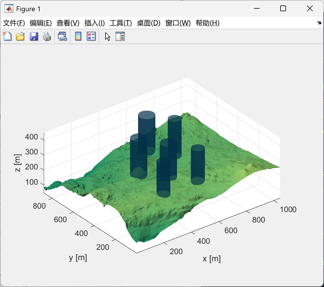 AI Visual Insight: This figure shows the 3D overlay between the mountain elevation mesh and the planned trajectory. It helps you inspect whether the path crosses ridgelines, avoids cylindrical threat regions, and maintains spatial continuity and a reasonable climb trend.
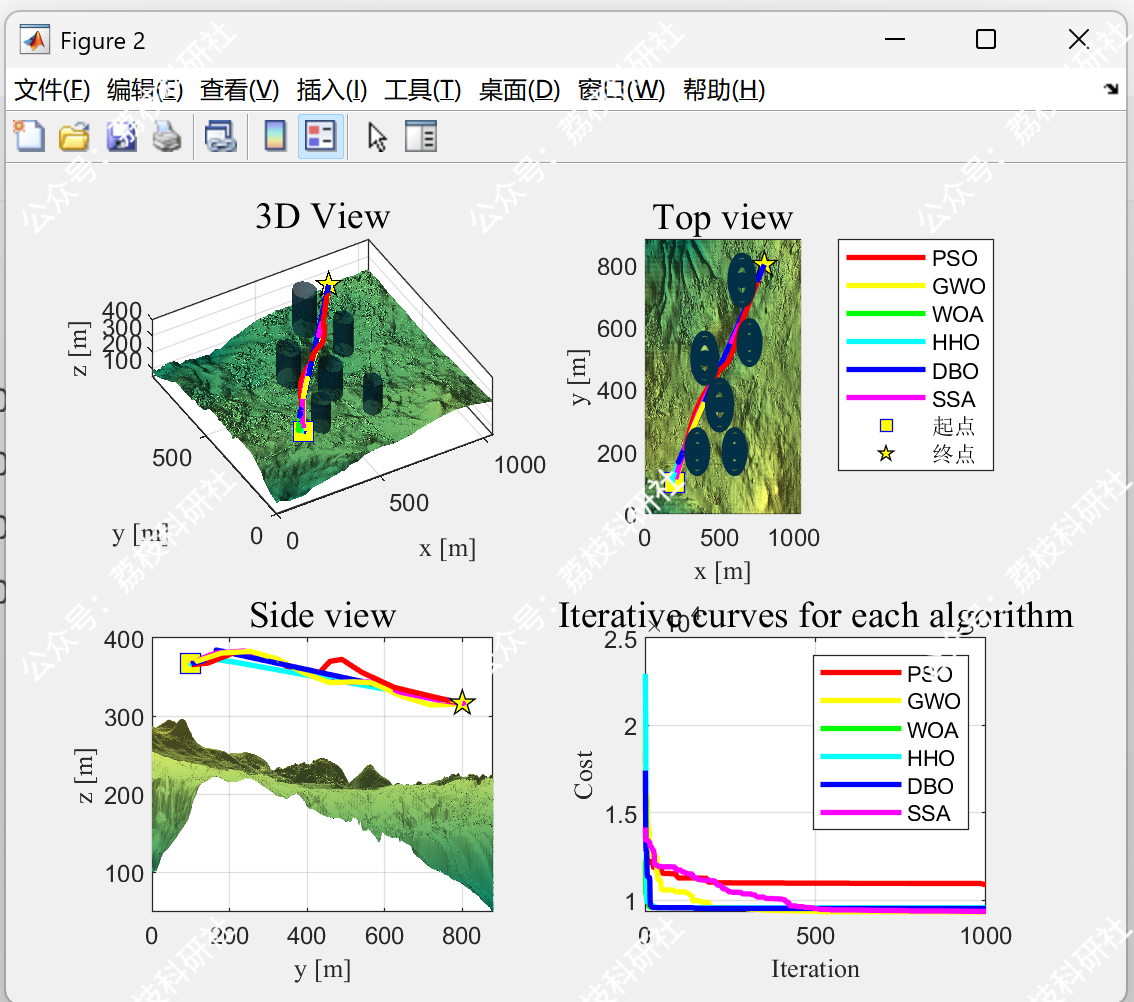 AI Visual Insight: This figure most likely presents a top-down view or a multi-path comparison view. It is useful for analyzing differences in obstacle-avoidance strategies across algorithms in planar projection, including turn density, safety margin from threat boundaries, and path redundancy.
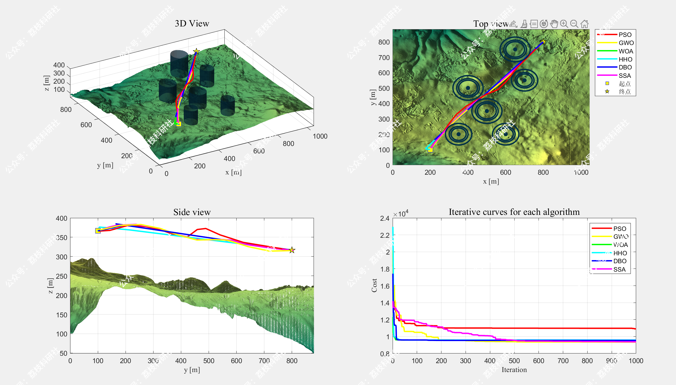 AI Visual Insight: This figure is typically used to present convergence curves or side-view altitude variation. It can help determine whether an algorithm converges prematurely, how convergence speeds differ across methods, and whether trajectory altitude consistently remains within a safe flight envelope.
function PlotModel(model)
    mesh(model.X, model.Y, model.H);              % Draw the 3D terrain mesh
    colormap(summer);                             % Set terrain color mapping
    shading interp;                               % Smooth surface shading
    material dull;                                % Reduce reflections to enhance mountain texture
    camlight left; lighting gouraud;              % Add lighting to improve depth perception
    hold on;

    threats = model.threats;                      % Load threat-region parameters
    for i = 1:size(threats,1)
        t = threats(i,:);                         % Extract a single threat
        [xc,yc,zc] = cylinder(t(4));              % Generate a cylinder from the radius
        xc = xc + t(1);                           % Translate to threat-center x
        yc = yc + t(2);                           % Translate to threat-center y
        zc = zc * 250 + t(3);                     % Scale and set height
        h = mesh(xc, yc, zc);                     % Draw the threat cylinder
        set(h,'edgecolor','none','facealpha',0.7); % Set transparency for easier path inspection
    end
end
This code renders mountain terrain and cylindrical threat zones to create the visualization environment for the path-planning experiment.
This research framework is better suited for algorithm validation than direct flight-control deployment
From a methodological perspective, this framework is highly suitable for paper reproduction, algorithm benchmarking, teaching demonstrations, and early-stage solution screening. Spherical-coordinate parameterization and a unified cost function allow different optimization algorithms to be evaluated fairly at the same abstraction level.
However, real deployment still requires additional capabilities, including dynamic obstacles, weather disturbances, communication links, energy-consumption models, and real-time replanning mechanisms. In other words, this is a high-quality offline planning and simulation framework, not a complete onboard navigation system.
Developers should prioritize three issues during implementation
First, confirm that the weight coefficients match the mission scenario. Inspection missions usually place more emphasis on path length and smoothness, while reconnaissance missions prioritize threat avoidance.
Second, verify that path-parameter bounds are consistent with vehicle performance. Maximum turn angle, maximum climb rate, and minimum ground clearance should not remain only at the simulation level.
Third, evaluate mean and variance across multiple runs instead of only reporting a single best result. The engineering value of swarm-intelligence algorithms depends heavily on stability.
FAQ
1. Why is spherical-coordinate parameterization more suitable than direct waypoint optimization for mountain path planning?
Spherical coordinates compress each path segment into three variables—step length, elevation angle, and azimuth angle—which significantly reduces dimensionality and naturally supports turning and climb constraints. This improves both convergence efficiency and trajectory feasibility.
2. Why do newer algorithms usually perform better among the six compared methods?
HHO, DBO, and SSA are generally stronger at balancing exploration and exploitation, coordinating population roles, and escaping local optima. As a result, they are more likely to find better and more stable feasible paths in complex non-convex constrained spaces.
3. Can this MATLAB method be used directly for real UAV flight?
It can serve as a strong foundation for offline planning and algorithm validation, but it cannot directly replace a flight-control system. Real-world deployment still requires dynamic obstacles, sensor error handling, wind-field disturbances, energy constraints, and online replanning.
Core Summary
This article reconstructs a 3D UAV path planning solution for complex mountainous scenarios. Its core components include spherical-coordinate path parameterization, joint terrain and threat modeling, a four-objective cost-function design, and a unified comparison framework for six intelligent optimization algorithms—PSO, GWO, WOA, HHO, DBO, and SSA—combined with MATLAB visualization to show path quality and convergence performance.