Multi-UAV Cooperative Transport Path Planning and Dynamic Control: RRT, EKF, and MATLAB Implementation

For multi-UAV cooperative transport missions, this article distills a reproducible solution: use 3D RRT for obstacle avoidance in complex environments, coordinate dual-UAV handoff with hierarchical control, and apply an EKF to estimate unknown payload mass online for better control accuracy. It addresses three core challenges: obstacle avoidance, synchronization, and payload uncertainty. Keywords: multi-UAV cooperation, RRT, EKF.

Technical Specifications at a Glance

Parameter	Description
Primary Language	MATLAB
Simulation Environment	Unity + MATLAB
Core Algorithms	3D RRT, seventh-order polynomial trajectory smoothing, EKF
Control Architecture	Mission layer + path layer + low-level control layer
Cooperation Mode	Dual-UAV synchronized pickup / handoff / transport
Payload Setup	Unknown-mass target with online estimation
GitHub Stars	Not provided in the source material
Core Dependencies	MATLAB numerical computing, collision detection, 3D environment modeling

This is a cooperative control solution for complex 3D transport scenarios

This solution focuses on two UAVs cooperatively transporting an object with unknown mass. The system goal is not simply to reach a destination, but to complete a three-stage mission—pickup, handoff, and transport—within a 3D space that includes both static and dynamic obstacles.

Compared with single-UAV transport, a cooperative approach improves payload capacity and mission redundancy, but it also introduces three critical challenges: path planning with obstacle avoidance, dual-UAV synchronization, and payload mass uncertainty. The value of the original material lies in the fact that it provides a relatively complete hierarchical implementation framework.

Hierarchical control is the key to stable deployment

The mission planning layer defines stage objectives such as approaching the target, completing pickup, reaching the handoff point, and continuing transport. The path planning layer generates collision-free paths using 3D RRT, while the low-level control layer tracks the trajectory and adjusts control inputs in real time based on payload changes.

The advantage of this structure is clear separation of responsibilities. The upper layer decides where to go, the middle layer decides how to avoid obstacles, and the lower layer decides how to fly there stably while carrying the payload.

3D RRT quickly produces feasible paths in obstacle-rich environments

The core of RRT is random sampling and tree expansion. It does not enforce global optimality, but it can find a feasible path quickly in complex spaces, which makes it well suited to the real-time requirements of multi-UAV transport tasks.

In the original implementation, delta sets the expansion step size, range_goal determines whether a new node is close enough to the goal, and check_line controls the sampling density for line-segment collision checking. Together, these parameters affect both planning speed and path feasibility.

% Core RRT parameter settings
a = 4000;          % Number of internal iterations; determines search completeness
delta = 5;         % Tree expansion step size; affects search speed and precision
range_goal = 3;    % Goal radius; reaching this range counts as arrival
check_line = 5;    % Number of samples for line-segment collision checking

start = travel(GENERAL,1:3);   % Start point of the current mission segment
goal  = travel(GENERAL,4:6);   % End point of the current mission segment

[NODELIST, PATH, COORD_PATH, found] = RRT(start, goal, a, ...
    meshes_vector, delta, check_line, range_goal); % Execute 3D RRT planning

This code generates a feasible 3D path for each mission segment while satisfying obstacle-avoidance constraints.

Seventh-order polynomial smoothing reduces control jitter caused by trajectory discontinuities

Paths generated directly by RRT are typically piecewise linear. That works well for search, but not for direct control. To avoid abrupt attitude changes at turning points, the original solution applies seventh-order polynomials to smooth transitions between path segments.

This method simultaneously constrains position, velocity, acceleration, and jerk at the start and end points, making the trajectory more continuous in higher-order derivatives. This step is especially important in payload transport scenarios, because payload swing can significantly amplify the effect of trajectory discontinuities.

% Boundary condition matrix for the seventh-order polynomial
A = [1 0 0 0 0 0 0 0;
     1 1 1 1 1 1 1 1;
     0 1 0 0 0 0 0 0;
     0 1 2 3 4 5 6 7;
     0 0 2 0 0 0 0 0;
     0 0 2 6 12 20 30 42;
     0 0 0 6 0 0 0 0;
     0 0 0 9 24 60 120 210];

b = [0 1 0 0 0 0 0 0]';      % Boundary constraints for position, velocity, acceleration, and jerk
ai = A \ b;                  % Solve for polynomial coefficients
s_t = ai(8)*lin.^7 + ai(7)*lin.^6 + ai(6)*lin.^5 + ai(5)*lin.^4 + ...
      ai(4)*lin.^3 + ai(3)*lin.^2 + ai(2)*lin + ai(1); % Generate the smooth parametric curve

This code constructs a time-parameterized curve with higher-order continuity for smooth connection between path points.

The trajectory can enter the control loop only after smoothing

The smoothed trajectory is interpolated segment by segment to generate PATH_TL, which is then tracked by the low-level controller. This significantly reduces abrupt changes in roll and pitch, improving stability and transport comfort.

The dual-UAV synchronization mechanism determines whether the handoff phase is reliable

In cooperative transport, the most fragile stage is usually not cruise flight, but handoff. The original solution uses a distance-threshold-based synchronization strategy: when the distance between the two UAVs is less than dsync, the first UAV releases the object and the second UAV immediately enters pickup mode.

The advantage of this mechanism is implementation simplicity, which makes it easy to validate in engineering prototypes. However, it is sensitive to position estimation, communication delay, and control error, so the low-level PID or attitude control loop must compensate for those errors.

if norm(pos_uav1 - pos_uav2) < dsync   % The distance between the two UAVs is below the synchronization threshold
    release_flag = 1;                  % The first UAV releases the payload
    pickup_flag  = 1;                  % The second UAV starts pickup
    m2_est = m1_est;                   % Inherit the mass estimate from the previous phase
end

This code triggers the dual-UAV handoff and switches the payload state and estimation variables inside the control state machine.

EKF removes the unknown payload from the controller’s blind spot

When transporting an object with unknown mass, using a fixed thrust parameter can easily cause altitude error, attitude overshoot, or even instability. To address this, the solution introduces an EKF to estimate target mass online and continuously update that estimate during transport.

The state variables can include mass, velocity, and acceleration, while observations come from the relationship between thrust and system kinematics. In essence, this turns payload mass from a fixed constant into a state that can be corrected online, improving how well the controller matches the true system dynamics.

AI Visual Insight: The figure shows the state update expression of the Extended Kalman Filter. Its core components include the prior state, Kalman gain, and observation residual, illustrating how the system continuously corrects the mass estimate through sensor measurements so that control parameters converge in real time as the payload changes.

% Update thrust based on mass estimation
m_hat = m_est(k);                  % Current mass estimate
F = m_hat * (g + a_ref);           % Compute the required thrust from the desired acceleration
u_thrust = thrust_allocation(F);   % Allocate thrust to each actuator

This code feeds the mass estimate output by the EKF directly back into the thrust controller, enabling dynamic control gain adjustment.

Experimental results show strong value for research reproduction

The reported results include an average planning time of about 2.3 seconds, dual-UAV handoff error below 0.5 meters, synchronization time below 3 seconds, mass estimation converging close to the true value in about 10 seconds, and steady-state error below 0.2 kilograms.

These metrics show that the solution reaches a verifiable level across three critical dimensions: it can plan, it can hand off, and it can converge. That makes it suitable for paper reproduction, course projects, and control algorithm prototyping.

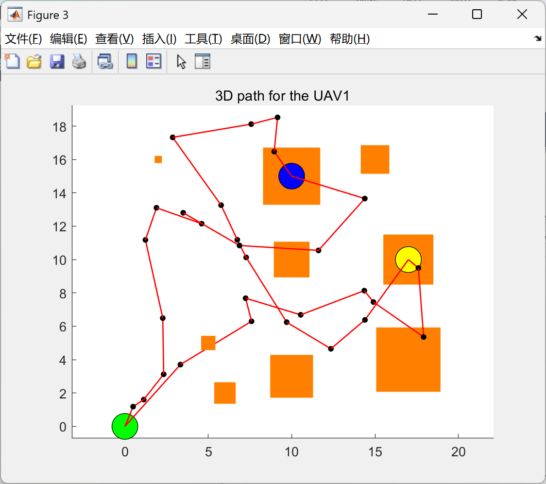
AI Visual Insight: The image shows path search results or flight-state distribution in a 3D simulation environment. It typically reveals obstacle layout, start and goal positions, and how the trajectory traverses space, helping validate whether the RRT-generated path satisfies obstacle-avoidance and reachability constraints.

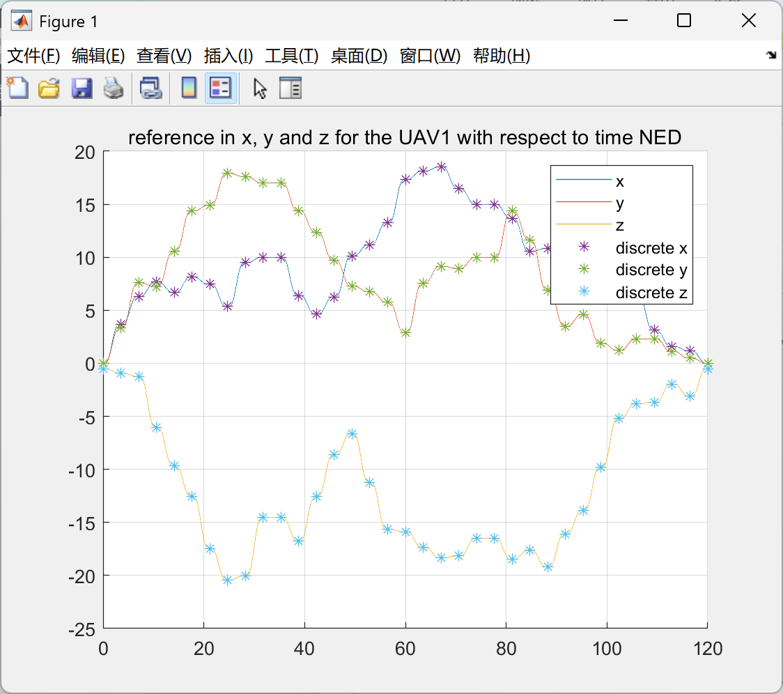
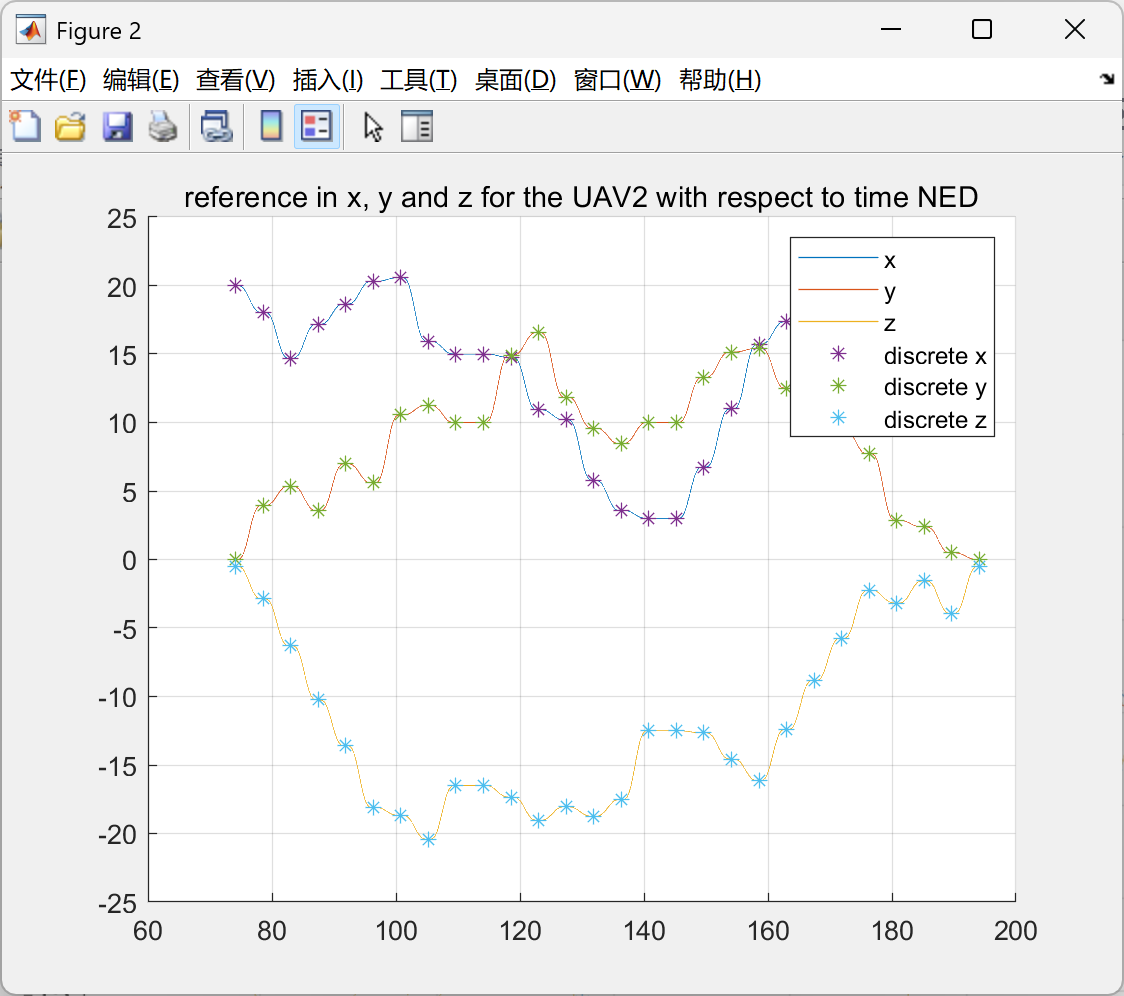AI Visual Insight: The image reflects trajectory or state evolution in another phase, possibly corresponding to a different mission segment or viewpoint of the smoothed path. It is mainly used to evaluate trajectory continuity and the quality of spatial turning behavior.

AI Visual Insight: The figure should show the relative positions of the UAVs and environmental obstacles, which helps assess whether the planned path preserves sufficient safety margin and whether there is any potential collision risk near the handoff point.

The current solution still has three clear upgrade paths

First, local replanning can be upgraded to online receding-horizon optimization to improve handling of dynamic obstacles and multi-UAV mutual avoidance. Second, RRT* or PRM can be introduced to improve path quality. Third, the 3D visualization can be enhanced to improve interpretability and demonstration value.

FAQ

Q1: Why prioritize RRT here instead of using RRT* directly?

A1: RRT emphasizes finding a feasible solution quickly, which makes it a better choice for first validating whether the full cooperative transport loop works end to end. If the next goal is to reduce flight distance, curvature, or energy consumption, switching to RRT* becomes more reasonable.

Q2: Where does online mass estimation improve control performance the most?

A2: The main improvement appears in thrust allocation and attitude-control matching. The closer the mass estimate is to the true value, the more stable altitude hold becomes, and the smaller the overshoot and oscillation during handoff.

Q3: How far is this MATLAB solution from deployment on real UAV hardware?

A3: It already has strong value for algorithm validation, but real-world deployment still requires additional engineering work, including sensor noise modeling, communication delay compensation, flight-controller interface adaptation, and safety redundancy design.

Core Summary: This article reconstructs a technical solution for multi-UAV cooperative payload transport. The core elements include 3D RRT obstacle-avoidance path planning, dual-UAV synchronized handoff, EKF-based online payload mass estimation, and key MATLAB simulation implementation details. It is well suited for research reproduction and engineering prototype validation.