For object detection training pipelines, this article organizes the core families of image data augmentation: geometric and pixel-level transforms, occlusion simulation, cross-sample mixing, and feature-level augmentation. These techniques address common pain points such as limited data, heavy occlusion, complex backgrounds, and poor learnability of small objects. Keywords: object detection, data augmentation, Mosaic.
Technical Specification Snapshot
| Parameter | Description |
|---|---|
| Task Domain | Object Detection / Instance Segmentation / Visual Perception |
| Primary Language | Python |
| Common Libraries | OpenCV, NumPy, PyTorch |
| Typical Frameworks | YOLO family, Albumentations pipelines |
| Core License | CC 4.0 BY-SA (as declared in the original source) |
| Stars | Not provided in the original content |
| Core Dependencies | cv2, numpy, torch |
Data augmentation defines the upper bound of detector generalization
In object detection, data augmentation is not a secondary trick. It is a tool for designing the training distribution. Its essence is to expose the model to more visual variations that are reasonable but absent from the limited dataset.
When the training set is small, class distribution is imbalanced, or the capture environment is too uniform, the model can easily overfit to background, lighting, and viewpoint. The role of augmentation is to expand the perturbation space of the input and improve robustness and transferability.
Geometric and pixel augmentation form the lowest-cost baseline
The most basic category of augmentation includes geometric transforms and pixel-level transforms. They do not change the semantic label, but they do change the appearance conditions of the target, teaching the model to ignore non-essential differences.
import cv2
import numpy as np

def aug_geometric(img: np.ndarray) -> dict:
    h, w = img.shape[:2]
    results = {}
    results["HorizontalFlip"] = cv2.flip(img, 1)  # Horizontal flip to simulate left-right viewpoint changes
    results["VerticalFlip"] = cv2.flip(img, 0)    # Vertical flip for augmentation in specific scenarios

    M = cv2.getRotationMatrix2D((w // 2, h // 2), 45, 1.0)
    results["Rotate45"] = cv2.warpAffine(img, M, (w, h))  # Rotate the object orientation

    crop = img[int(h * 0.15):int(h * 0.85), int(w * 0.15):int(w * 0.85)]
    results["CenterCrop70%"] = cv2.resize(crop, (w, h))   # Crop and rescale to simulate close-range variation
    return results
This code demonstrates flipping, rotation, and crop-resize. Its core value lies in improving viewpoint invariance.
 AI Visual Insight: The figure applies horizontal flip, vertical flip, rotation, and center crop with resampling to the same target. You can directly observe changes in contour position, orientation, and scale while the semantics remain unchanged. This shows that geometric augmentation mainly improves tolerance to pose and viewpoint shifts.
def aug_color_jitter(img: np.ndarray) -> dict:
    hsv = cv2.cvtColor(img, cv2.COLOR_RGB2HSV).astype(np.float32)
    results = {}
    results["Brightness+60"] = np.clip(img.astype(np.float32) + 60, 0, 255).astype(np.uint8)  # Increase brightness
    results["Contrastx1.8"] = np.clip(img.astype(np.float32) * 1.8, 0, 255).astype(np.uint8)   # Increase contrast

    sat = hsv.copy()
    sat[..., 1] = np.clip(sat[..., 1] * 2, 0, 255)  # Amplify the saturation channel
    results["Saturationx2"] = cv2.cvtColor(sat.astype(np.uint8), cv2.COLOR_HSV2RGB)
    return results
This code simulates different exposure levels, contrast, and color styles. It is well suited to scenarios with strong lighting variation.
 AI Visual Insight: The figure shows distribution differences after changes in brightness, contrast, saturation, and hue. The main object remains the same, while the color statistics change significantly. This type of augmentation reduces the model’s dependence on color bias tied to a specific camera, weather condition, or time of day.
Noise and occlusion augmentation directly improve robustness in complex scenes
Real deployment environments often include noise, occlusion, stains, and partial corruption. If training uses only clean data, false positives and missed detections usually increase noticeably after deployment.
def aug_noise(img: np.ndarray) -> dict:
    results = {}
    gauss = np.random.normal(0, 25, img.shape).astype(np.float32)
    results["GaussianNoise"] = np.clip(img.astype(np.float32) + gauss, 0, 255).astype(np.uint8)  # Gaussian noise
    return results
This code uses Gaussian noise to simulate sensor perturbation and image degradation under low-light conditions.
 AI Visual Insight: Grain noise covers both object and background texture, and some edge detail is submerged. This reflects how noise augmentation trains the model to capture stable structural features even under low signal-to-noise conditions.
def aug_random_erasing(img: np.ndarray, ratio: float = 0.15) -> np.ndarray:
    out = img.copy()
    h, w = out.shape[:2]
    eh, ew = int(h * ratio), int(w * ratio)
    top = np.random.randint(0, h - eh)
    left = np.random.randint(0, w - ew)
    out[top:top + eh, left:left + ew] = 128  # Randomly erase a local region
    return out
This code applies local occlusion to force the model to recover target semantics from the remaining visible context.
 AI Visual Insight: Part of the object is covered by a regular rectangle, removing key texture cues while preserving the overall context. This training approach reduces overfitting to a single local texture pattern.
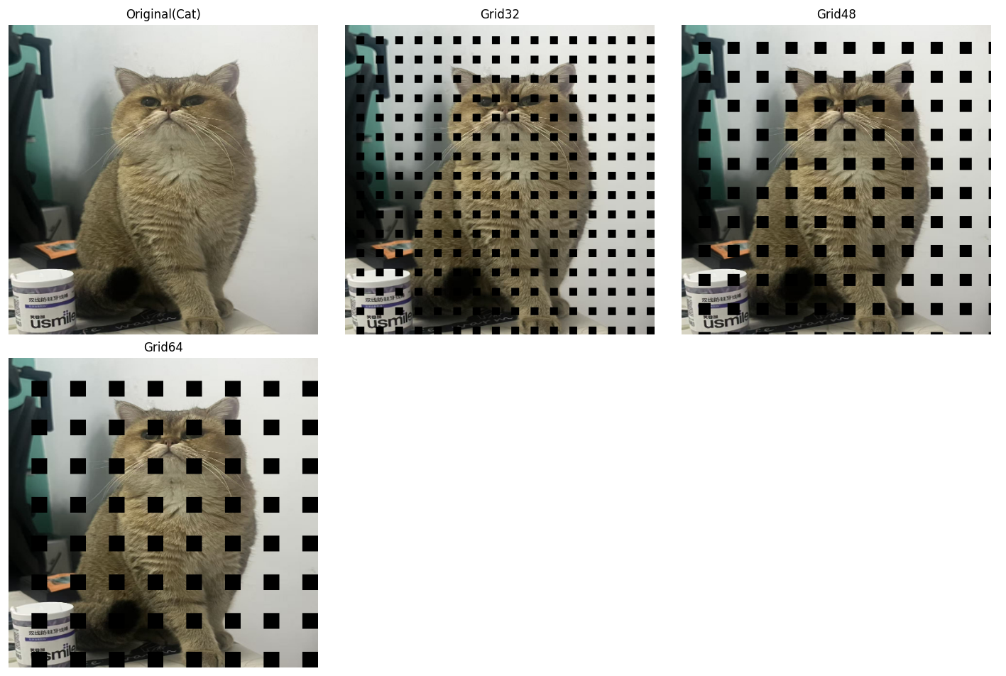 AI Visual Insight: The regular grid-like occlusion periodically interrupts both object texture and background continuity while preserving some global contour information. The value of GridMask is that it encourages the model to prioritize overall object structure instead of local high-frequency textures.
Cross-sample mixing augmentation has become standard in the YOLO ecosystem
When single-image augmentation is no longer enough to expand the distribution, cross-sample mixing becomes a stronger option. It no longer operates on just one image. Instead, it directly recomposes pixels and labels from multiple images.
def aug_mixup(img_a: np.ndarray, img_b: np.ndarray, alpha: float = 0.4) -> np.ndarray:
    lam = np.random.beta(alpha, alpha)
    mixed = lam * img_a.astype(np.float32) + (1 - lam) * img_b.astype(np.float32)  # Linearly blend two images
    return np.clip(mixed, 0, 255).astype(np.uint8)
This code overlays two images with transparency, improving class-boundary smoothness and generalization.
 AI Visual Insight: The figure transparently blends two scenes so that foreground and background coexist. This shows how Mixup reduces the model’s incorrect reliance on single-scene priors and background co-occurrence patterns.
def aug_cutmix(img_a: np.ndarray, img_b: np.ndarray, cut_ratio: float = 0.3) -> np.ndarray:
    out = img_a.copy()
    h, w = out.shape[:2]
    ch, cw = int(h * cut_ratio), int(w * cut_ratio)
    top = np.random.randint(0, h - ch)
    left = np.random.randint(0, w - cw)
    out[top:top + ch, left:left + cw] = img_b[top:top + ch, left:left + cw]  # Paste a local patch from another image
    return out
This code pastes a local region from another image into the current image, which is useful for learning occlusion and improving boundary sensitivity.
 AI Visual Insight: A local region is replaced with a patch from a different source image, creating strong boundaries and a mixed-object structure. CutMix not only increases occlusion samples, but also strengthens the detector’s ability to handle box edges and conflicting local context.
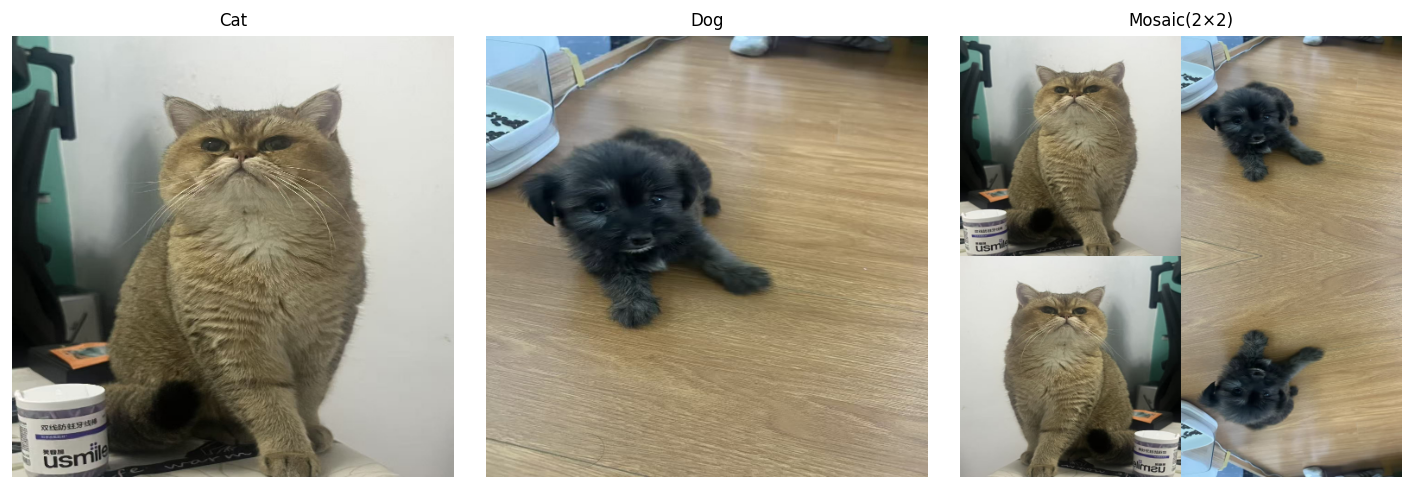 AI Visual Insight: The image is assembled from four sub-images and then resized to a unified shape, significantly increasing object density and background diversity within a single training sample. Mosaic is especially effective for small object detection because it brings more objects at different scales into the same receptive field.
Advanced augmentation methods fit long-tail classes and lightweight models better
Copy-Paste is an efficient method for handling long-tail classes in instance segmentation and object detection. It copies object regions and places them elsewhere, quickly increasing the occurrence frequency of rare classes.
def aug_copy_paste(src: np.ndarray, dst: np.ndarray, obj_ratio: float = 0.25) -> np.ndarray:
    out = dst.copy()
    h, w = src.shape[:2]
    oh, ow = int(h * obj_ratio), int(w * obj_ratio)
    cy, cx = h // 2, w // 2
    obj = src[cy - oh // 2:cy + oh // 2, cx - ow // 2:cx + ow // 2]  # Crop the center object region
    top = np.random.randint(0, max(out.shape[0] - oh, 1))
    left = np.random.randint(0, max(out.shape[1] - ow, 1))
    out[top:top + oh, left:left + ow] = obj  # Paste it at a random location in the target image
    return out
This code demonstrates a simplified Copy-Paste augmentation. Its essence is to resample the spatial distribution of rare objects.
 AI Visual Insight: A local object from the source image is extracted and pasted into a different background, changing the co-occurrence relationship between object and scene. This shows that Copy-Paste is a direct and effective solution for long-tail classes and background binding issues.
Feature-level augmentation lifts perturbation from pixel space to semantic space
ISDA does not directly modify the original image. Instead, it introduces statistical perturbation in feature space. By estimating the covariance of class features, it constructs reasonable semantic perturbations and is particularly suitable for improving lightweight models.
import torch
import torch.nn as nn

class ISDALoss(nn.Module):
    def __init__(self, estimator):
        super().__init__()
        self.estimator = estimator

    def forward(self, features, y, target_layer):
        self.estimator.update_CV(features, y)  # Update feature statistics for each class
        logits = target_layer(features)
        logits = logits + self.estimator.get_purturb(features, y)  # Inject feature-level perturbation compensation
        return nn.CrossEntropyLoss()(logits, y)
This code shows that ISDA is integrated into the loss computation stage, using feature distributions to approximate virtual augmented samples.
Augmentation strategy should be matched to business pain points instead of blindly stacked
More augmentation is not always better. Better matching is what matters. If the task is dominated by small objects, prioritize Mosaic, random cropping, and multi-scale training. If occlusion is severe, increase the use of CutMix, Random Erasing, and GridMask.
If the dataset is extremely small and class imbalance is obvious, Copy-Paste and Mixup are more valuable. If compute is limited but you still want better generalization, feature-level augmentation such as ISDA is a good training-time compensation. In engineering practice, start with basic augmentation, then gradually introduce stronger augmentation while monitoring changes in mAP and recall.
FAQ
Q1: Which data augmentations are most worth enabling first in object detection?
A: Usually horizontal flip, color jitter, random crop, and Mosaic. They provide stable gains, are easy to implement, and work especially well for YOLO-style models.
Q2: How should I choose between Mixup, CutMix, and Mosaic?
A: Mixup is good for improving generalization and smoothing classification boundaries. CutMix is more suitable for occlusion learning and boundary awareness. Mosaic is the most effective for small objects and complex backgrounds, so it is often the first choice for detection tasks.
Q3: Why is ISDA suitable for lightweight models?
A: Because it does not rely on a large number of pixel-level augmented samples. Instead, it uses feature distributions to construct implicit augmentation, improving feature robustness and classification boundary stability at lower training cost.
Core Summary: This article systematically reconstructs the image data augmentation landscape for object detection, covering geometric transforms, color jitter, noise injection, occlusion augmentation, Mixup, CutMix, Mosaic, Copy-Paste, and ISDA. It combines code examples with augmentation selection guidance to explain their impact on robustness, generalization, and small object detection performance.