Pandas concat vs merge vs join: A Practical Guide to Data Combination Rules - Devuly | Smart Analytics for Developers & Projects

Pandas data combination is a critical step before data cleaning and modeling. This article focuses on three connection mechanisms—concat, merge, and join—and explains row and column concatenation, key-based merging, index alignment, and duplicate-column handling. It addresses common pain points such as how to combine data, which keys or axes control the result, and why rows increase or missing values appear. Keywords: Pandas, concat, merge.

Table of Contents

Technical Specification Snapshot

Parameter	Description
Language	Python
Core library	pandas
Data structures	Series, DataFrame
Combination patterns	concat, merge, join
Underlying dependency	NumPy
Applicable scenarios	Data cleaning, feature concatenation, wide-table merging
Star count	Not provided in the source
License	pandas is BSD-3-Clause; project license not provided in the source

Pandas data combination falls into concatenation and relational merging

In Pandas, concat behaves more like stacking along an axis and emphasizes alignment by index or column name. merge is closer to a database join and emphasizes relational combination based on keys. join is a DataFrame-oriented convenience interface for index-based alignment.

Understanding the differences between these three methods directly reduces issues such as unexpected missing values, explosive row growth from duplicate matches, and column conflicts being overwritten. In real projects, most preprocessing errors happen during the combine stage, not during modeling.

concat works best for batch concatenation of similarly structured data

By default, concat combines along axis=0, which makes it suitable for vertically appending multiple Series or DataFrames. If the input objects have different indexes, Pandas preserves the original indexes, so the result can contain duplicate index values.

import pandas as pd

s1 = pd.Series(["A", "B"], index=[1, 2])
s2 = pd.Series(["D", "E"], index=[4, 5])

result = pd.concat([s1, s2])  # Concatenate by rows by default, axis=0
print(result)

This example shows the most basic vertical concatenation behavior. The result preserves the original indexes.

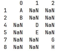
When concatenating by columns, set axis=1. In this case, Pandas aligns by index and automatically fills missing positions with NaN. This is also the first place many developers encounter missing values.

import pandas as pd

s1 = pd.Series(["A", "B"], index=[1, 2])
s2 = pd.Series(["D", "E"], index=[4, 5])

result = pd.concat([s1, s2], axis=1)  # Concatenate by columns with automatic index alignment
print(result)

This example shows that column-wise concatenation is essentially outer-join-style alignment by index.

AI Visual Insight: The image shows the tabular result after concatenating two Series by columns. The indexes are unified into multiple discrete values, and unmatched positions are filled with NaN, clearly illustrating the index alignment behavior of concat(axis=1).

Concatenating a DataFrame and a Series requires attention to names and axis direction

When a DataFrame and a Series are concatenated by rows, the Series is treated as an independent record or object fragment, which can produce structural inconsistencies in the result. When concatenated by columns, the Series name becomes the column name, and it may duplicate an existing column name.

import pandas as pd

df = pd.DataFrame({"a": [1, 2], "b": [4, 5]}, index=[1, 2])
s = pd.Series([7, 10], index=[1, 2], name="a")

result = pd.concat([df, s], axis=1)  # The Series name becomes the new column name
print(result)

This example shows that Pandas does not automatically resolve column name conflicts when concatenating a DataFrame and a Series horizontally.

ignore_index can rebuild a continuous index after vertical concatenation

If the original index has no business meaning and only acts as a placeholder, preserving it after concatenation often makes later filtering more complex. In this case, use ignore_index=True.

import pandas as pd

df1 = pd.DataFrame({"a": [1, 2], "b": [4, 5]}, index=[1, 2])
df2 = pd.DataFrame({"a": [7, 8], "b": [10, 11]}, index=[1, 2])

result = pd.concat([df1, df2], ignore_index=True)  # Reset to a continuous integer index
print(result)

This example rebuilds a clean index after appending data in batches.

The join parameter controls set logic on the non-concatenation axis in concat

Another often overlooked aspect of concat is how it handles columns or indexes on the axis other than the main concatenation axis. By default, join="outer" keeps the union, while join="inner" keeps the intersection.

import pandas as pd

df1 = pd.DataFrame({"a": [1, 2], "b": [4, 5]})
df2 = pd.DataFrame({"b": [7, 8], "c": [10, 11]})

result = pd.concat([df1, df2], join="inner")  # Keep only the shared column b
print(result)

This example shows that concat can also express filtering semantics such as keeping only the shared columns.

merge is better suited for relational data combination based on keys

When two tables are related by business primary keys, foreign keys, or semantically equivalent fields, prefer merge. It is the closest Pandas operation to SQL joins and is ideal for modeling relationships across entities such as orders, users, departments, and tags.

merge supports one-to-one, many-to-one, and many-to-many relationships

A one-to-one merge is suitable for adding attribute fields. A many-to-one merge is common when joining a fact table to a dimension table. A many-to-many merge creates Cartesian expansion, so handle it with extra care because the resulting row count can greatly exceed expectations.

import pandas as pd

df1 = pd.DataFrame({"employee": ["Bob", "Jake", "Lisa", "Sue"],
                    "group": ["Accounting", "Engineering", "Engineering", "HR"]})
df2 = pd.DataFrame({"group": ["Accounting", "Engineering", "Engineering", "HR"],
                    "skills": ["math", "coding", "linux", "organization"]})

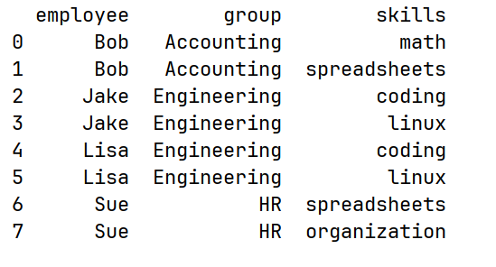
result = pd.merge(df1, df2, on="group")  # Merge on the business key group
print(result)

This example demonstrates relational expansion when duplicate values exist in the shared key.

AI Visual Insight: The image shows the result of merging an employee table and a skills table on the group field. The same group matches multiple times, which produces a many-to-many expansion and clearly demonstrates the Cartesian product risk of merge.

merge can explicitly use column names or indexes as join keys

If both sides use the same field name, on is the most direct option. If the field names differ, use left_on and right_on. If the keys are already set as indexes, use left_index=True and right_index=True.

import pandas as pd

left = pd.DataFrame({"employee": ["Bob", "Jake", "Lisa"],
                     "group": ["A", "B", "B"]})
right = pd.DataFrame({"name": ["Bob", "Jake", "Lisa"],
                      "salary": [70000, 80000, 120000]})

result = pd.merge(left, right, left_on="employee", right_on="name")  # Map and merge across different column names
print(result)

This example shows that tables with different naming systems can still be linked accurately.

The how parameter determines whether to keep the intersection or union

By default, merge uses inner, which keeps only the keys that appear in both tables. If you want to preserve as much information as possible, use outer. If you want to enrich records using the left table as the base, use left. Use right when the right table is the base.

import pandas as pd

df1 = pd.DataFrame({"name": ["Peter", "Paul", "Mary"], "food": ["fish", "beans", "bread"]})
df2 = pd.DataFrame({"name": ["Mary", "Joseph"], "drink": ["wine", "beer"]})

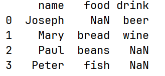
result = pd.merge(df1, df2, how="outer", on="name")  # Keep all names from both sides
print(result)

This example shows how an outer join preserves the full set of entities and fills missing attributes with NaN.

AI Visual Insight: The image presents the result of an outer join. Unmatched entities from both the left and right tables are preserved, and missing attributes are represented with NaN, clearly showing the union-preserving strategy of how="outer".

Duplicate column names and the join method require explicit conflict management

When two DataFrames contain non-key columns with the same name, merge automatically appends the suffixes _x and _y. This default behavior works, but it is not very readable in production code. It is better to define explicit names through suffixes.

import pandas as pd

df1 = pd.DataFrame({"name": ["Bob", "Jake"], "rank": [1, 2]})
df2 = pd.DataFrame({"name": ["Bob", "Jake"], "rank": [3, 1]})

result = pd.merge(df1, df2, on="name", suffixes=("_left", "_right"))  # Customize suffixes for conflicting columns
print(result)

This example ensures that duplicate columns keep clear semantics after the merge.

join is a convenience method on DataFrame. Under the hood, it is still a merge-like operation, but it is more oriented toward index alignment. If columns overlap, use lsuffix and rsuffix to avoid naming conflicts.

In real projects, choose concat, merge, and join based on the shape of the problem

If you are appending logs, sample sets, or partitioned files in batches, use concat first. If you are linking user tables, order tables, and tag tables by business keys, use merge first. If your key is already the index, or you simply want to align two DataFrames quickly by index, join is more concise.

A practical rule of thumb is this: as soon as you start asking, “What is the primary key?”, you should reach for merge instead of concat.

FAQ

FAQ 1: Why do I get many NaN values after concatenating by columns with concat?

Because concat(axis=1) aligns by index. When the indexes differ across objects, unmatched positions are automatically filled with NaN. This is not an error. It is the normal behavior of outer-join-style alignment.

FAQ 2: Why does the merged result contain far more rows than the original tables?

This usually means you created a many-to-many merge. As long as the join key contains duplicate values in both the left and right tables, merge expands into a Cartesian product. Check key uniqueness first, then decide whether deduplication is required.

FAQ 3: When should I use join instead of merge?

Use join when the join key is already stored in the index, or when you only need a quick index-based column alignment. If you need to map different column names, control complex keys, or switch among multiple join strategies, merge is more general.

Core summary: This article systematically reconstructs the core usage patterns of Pandas data combination functions. It focuses on the differences among concat, merge, and join across Series, DataFrame, multi-key combination, index-based joins, and duplicate-column handling, helping developers build a reliable mental model for data concatenation and merging.