PyTorch Fully Connected Neural Network Example: From Layer Definitions to Parameter Counting - Devuly | Smart Analytics for Developers & Projects

[AI Readability Summary]

This article walks through a PyTorch fully connected neural network example, covering model structure, forward propagation, weight initialization, and parameter counting. It helps beginners understand layer dimensions, activation functions, and Softmax outputs. Keywords: PyTorch, fully connected neural network, parameter initialization.

Table of Contents

Technical specifications are summarized below

Parameter	Details
Primary Language	Python
Core Framework	PyTorch
Network Type	Multilayer Perceptron (MLP) / Fully Connected Neural Network
Input Dimension	3
Output Dimension	2
Activation Functions	Sigmoid, ReLU, Softmax
Initialization Strategy	Xavier Normal, Kaiming Normal
Core Dependencies	torch, torch.nn, torchsummary
License	The original page shows CC 4.0 BY-SA
Star Count	Not provided in the original source

This example demonstrates a minimal and interpretable neural network architecture

This network consists of three linear layers: the first layer is 3→3, the second layer is 3→2, and the output layer is 2→2. Its value does not come from complexity, but from connecting the four most essential parts of a neural network into one clear example: defining layers, configuring activations, running forward propagation, and understanding the output.

Compared with directly using higher-level abstractions, this handwritten nn.Module approach is better suited for learners who want to build model intuition, especially around how output dimensions change across layers and why the final output becomes a probability distribution.

The core network configuration is as follows

import torch
import torch.nn as nn

class MyModel(nn.Module):
    def __init__(self):
        super().__init__()
        self.layer1 = nn.Linear(3, 3)   # First hidden layer: input 3 dimensions, output 3 dimensions
        self.layer2 = nn.Linear(3, 2)   # Second hidden layer: input 3 dimensions, output 2 dimensions
        self.layer3 = nn.Linear(2, 2)   # Output layer: input 2 dimensions, output 2 dimensions

This code defines the network skeleton, which serves as the foundation for forward propagation and training.

Different layers use different initialization methods and activation functions to stabilize training

The original example provides a clear initialization strategy: the first layer and the output layer use Xavier initialization, while the second layer uses He initialization. This pairing aligns with the activation functions: Sigmoid is commonly paired with Xavier, while ReLU is commonly paired with He, helping reduce the risk of vanishing gradients or unstable variance.

Although PyTorch initializes parameters by default, explicit initialization is more instructive in teaching, experiment reproduction, and convergence debugging scenarios.

An optional way to initialize parameters is shown below

import torch.nn.init as init

# Xavier is better suited for Sigmoid/Tanh-style activations
init.xavier_normal_(self.layer1.weight)   # Initialize first-layer weights
init.zeros_(self.layer1.bias)             # Zero the bias

# He is better suited for ReLU-style activations
init.kaiming_normal_(self.layer2.weight)  # Initialize second-layer weights
init.zeros_(self.layer2.bias)             # Zero the bias

# Continue using Xavier for the output layer
init.xavier_normal_(self.layer3.weight)   # Initialize output-layer weights
init.zeros_(self.layer3.bias)             # Zero the bias

This code explicitly controls the parameter distribution of each layer so that the initial training state better matches the behavior of the chosen activation functions.

The forward pass clearly shows the nonlinear modeling path

The forward propagation order in this model is: linear transformation → Sigmoid → linear transformation → ReLU → linear transformation → Softmax. The first two layers extract and compress features, and the final layer maps the result to probabilities for two classes.

Softmax(dim=-1) is the key concept here. It means normalization is applied along the last dimension, which corresponds to the class dimension for each sample. As a result, each row in the output sums to 1.

The full `forward` implementation is shown below

def forward(self, x):
    # x should have shape (batch_size, 3)
    x = torch.sigmoid(self.layer1(x))      # Apply Sigmoid after the first hidden layer
    x = torch.relu(self.layer2(x))         # Apply ReLU after the second hidden layer
    x = torch.softmax(self.layer3(x), dim=-1)  # Apply Softmax normalization along the last dimension
    print(x)                               # Print class probabilities for each sample
    return x

This code implements the full mapping from input features to classification probabilities.

The diagrams clearly explain layer connectivity and tensor shape changes

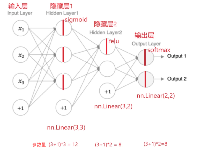AI Visual Insight: The diagram shows the data flow of a typical feedforward fully connected network. It starts with a 3-dimensional input, passes through the first hidden layer, compresses into a 2-dimensional hidden representation, and finally produces outputs for 2 classes. The visualization highlights the number of neurons in each layer and the linear mapping relationship, making it useful for understanding how in_features and out_features correspond.

Based on this structure, the tensor shape progression is straightforward: the input is (batch, 3), the first layer output remains (batch, 3), the second layer output becomes (batch, 2), and the final output is also (batch, 2).

Using `summary` makes the model structure easier to inspect

from torchsummary import summary

if __name__ == "__main__":
    model = MyModel()
    summary(model, input_size=(3,), device="cpu")  # Print parameter counts and shapes for each layer

This code prints the network structure, output sizes, and total parameter count, making it easy to quickly verify whether the model definition is correct.

The Softmax output confirms the classification semantics of the model

When the output looks like [0.3285, 0.6715], it means the model predicts a 0.3285 probability for the first class and a 0.6715 probability for the second class. These two values sum to 1, which is the direct result of Softmax normalization.

This type of output is typically passed to a cross-entropy loss function during training, but at the beginner stage, it is more important to first understand that the output is not a class label, but a probability distribution.

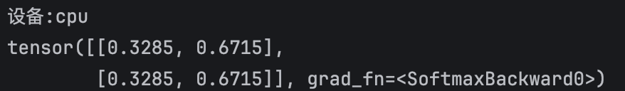AI Visual Insight: This screenshot shows the two-dimensional probability output after the model completes forward propagation. The two values sum to 1, indicating that the Softmax layer has normalized the output along the class dimension. This directly confirms that the task is binary classification probability prediction rather than regression.

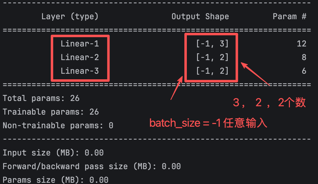AI Visual Insight: This figure shows tensor shapes and parameter statistics in the model summary. It emphasizes the placeholder meaning of the batch dimension -1, which indicates that the batch size is variable. It also shows that each layer output dimension strictly matches the linear layer’s out_features, which helps diagnose input dimension mismatch issues.

Parameter counting helps you quickly verify whether the layer design is correct

The parameter count formula for a fully connected layer is: input dimension × output dimension + output dimension bias.

Using this formula:

First layer: 3×3+3=12
Second layer: 3×2+2=8
Third layer: 2×2+2=6
Total parameter count: 12+8+6=26

If your manual calculation matches the summary output, the layer definitions and dimension design are usually correct. This is a very efficient self-check when debugging neural networks.

The following sample code manually verifies parameter counts

layers = [(3, 3), (3, 2), (2, 2)]
total = 0

for in_dim, out_dim in layers:
    params = in_dim * out_dim + out_dim   # Weight parameters + bias parameters
    total += params
    print(f"{in_dim}->{out_dim}: {params}")

print(f"Total params: {total}")          # Expected output: 26

This code independently validates the parameter count for each layer and for the full model.

This case works well as a PyTorch neural network starter template

It covers nn.Module inheritance, custom layers, forward propagation, activation function selection, initialization strategy, and parameter count calculation. Together, these topics include nearly all the essential concepts a beginner needs when writing a model by hand for the first time.

If you want to extend this into a full training workflow, you only need to add a loss function, an optimizer, and dataset iteration to turn it into a complete supervised learning project.

FAQ

1. Why does the output layer use Softmax instead of ReLU?

Softmax converts the output into a probability distribution, making it suitable for multiclass or binary classification probability modeling. ReLU only performs nonlinear truncation. It does not guarantee that outputs sum to 1, and it does not carry probabilistic meaning.

2. Why is He initialization more suitable for the second layer?

Because the second layer is followed by ReLU. He initialization better preserves variance stability during both forward and backward propagation, which helps reduce gradient decay issues in deeper networks.

3. What exactly does `dim=-1` mean in Softmax?

It means normalization is performed along the last dimension. For an output with shape (batch, 2), this means normalizing the two class scores for each sample so that each row becomes a probability distribution that sums to 1.

Core takeaway: This article uses a 3→3→2→2 PyTorch fully connected neural network example to clearly explain model definition, Xavier/He initialization, Sigmoid/ReLU/Softmax forward propagation, output dimensions, and parameter counting. It works well as a hands-on starter template for learning neural networks.