PyTorch LSTM Gold Price Forecasting: Feature Engineering, Time Series Modeling, and Error Analysis - Devuly | Smart Analytics for Developers & Projects

This article focuses on a PyTorch-based LSTM gold price forecasting project. Its core capability is to predict the next trading day’s closing price using historical gold prices and technical indicators, addressing the limitations of traditional statistical methods in modeling nonlinear market fluctuations. Keywords: LSTM, time series forecasting, gold price.

Table of Contents

Technical Specifications at a Glance

Parameter	Description
Language	Python 3.9
Deep Learning Framework	PyTorch
Data Source	Kaggle GoldUSD.csv
Task Type	Multivariate Time Series Regression
Input Window	30 trading days
Target	Next trading day closing price
Core Dependencies	pandas, numpy, torch, scikit-learn, matplotlib
Runtime Environment	Jupyter Notebook
Reported Metrics	MAE = 64.28, RMSE = 100.89, MAPE = 1.90%, R² = 0.9859
GitHub Stars	Not provided in the original source

This project builds a reusable financial time series forecasting pattern with LSTM

Gold prices are influenced by macroeconomic conditions, risk appetite, interest rate expectations, and market sentiment. As a result, the series exhibits clear nonlinear behavior. This project uses LSTM to capture long-term dependencies and enhances input representations with technical indicators.

The dataset spans from 2000-08-30 to 2026-03-03 and includes the fields Open, High, Low, Close, and Volume. Compared with univariate forecasting based only on closing prices, this multivariate setup is much closer to a real trading environment.

AI Visual Insight: The image presents the project cover and task theme, emphasizing that this experiment focuses on gold price time series forecasting. It is a typical financial regression problem rather than a classification or event detection task.

The data loading stage first guarantees chronological order and schema consistency

For time series tasks, disordered records and inconsistent fields are major risks. The original workflow first parses dates, sorts the rows, and standardizes column names, then prints the sample range and closing price distribution to prepare for sliding-window modeling.

import pandas as pd
import numpy as np
import torch

# Load the data and sort it in ascending date order
df = pd.read_csv("GoldUSD.csv")
df["Date"] = pd.to_datetime(df["Date"], dayfirst=True)  # The raw dates use day-month-year format
df = df.sort_values("Date").reset_index(drop=True)      # Time order must remain correct

df.columns = ["Date", "Open", "High", "Low", "Close", "Volume"]
print(df[["Date", "Close"]].head())

This code completes the most fundamental and most critical alignment step in time series modeling.

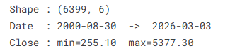AI Visual Insight: The image should show the basic dataset information output, such as sample dimensions, time span, and price range, to verify that the dataset covers a sufficiently long period and is suitable for training a long-dependency model.

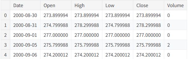AI Visual Insight: The image should display the data preview or the first few records, showing that the date field has been parsed successfully and that the OHLCV columns are structured consistently for downstream feature engineering and normalization.

Feature engineering converts raw market data into learnable signals with technical indicators

The project does not stop at raw OHLCV data. It adds derived features such as returns, trading range, moving averages, short-term volatility, momentum, and average volume. This step directly determines whether the model can learn trend, deviation, and volatility structure.

The target variable is defined as the next day’s closing price with Target=Close.shift(-1), turning the task into a standard supervised learning problem. Because rolling and shift introduce missing values, the pipeline cleans them consistently with dropna().

# Build key technical indicators
df["Return"] = df["Close"].pct_change()                 # Daily return
df["MA_5"] = df["Close"].rolling(5).mean()             # 5-day moving average
df["MA_20"] = df["Close"].rolling(20).mean()           # 20-day moving average
df["Volatility_5"] = df["Return"].rolling(5).std()     # 5-day volatility
df["Momentum_5"] = df["Close"] - df["Close"].shift(5) # 5-day momentum

df["Target"] = df["Close"].shift(-1)                   # Use the next trading day's close as the prediction target
df = df.dropna().reset_index(drop=True)

This code transforms a static market table into supervised learning samples designed for forecasting.

The sliding window converts a 2D table into the 3D tensor format required by LSTM

LSTM does not consume single-row features. It requires a continuous historical sequence. This project uses the previous 30 days as one window. Each sample has the shape (window, features), and the final dataset is assembled into (samples, window, features).

At the same time, features and targets are normalized separately with MinMaxScaler, then split into training, validation, and test sets in chronological order to avoid future information leakage. This is one of the most commonly overlooked but essential practices in financial time series work.

from sklearn.preprocessing import MinMaxScaler

WINDOW = 30
feature_scaler = MinMaxScaler()
target_scaler = MinMaxScaler()

X_scaled = feature_scaler.fit_transform(df[FEATURES].values)
y_scaled = target_scaler.fit_transform(df[["Target"]].values)

def build_sequences(X, y, window):
    Xs, ys = [], []
    for i in range(window, len(X)):
        Xs.append(X[i-window:i])  # Use the previous 30 days as the input sequence
        ys.append(y[i])           # The current sample maps to the next-day target value
    return np.array(Xs, dtype=np.float32), np.array(ys, dtype=np.float32)

This code defines the core transformation logic from tabular features to sequential training samples.

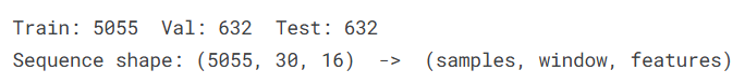AI Visual Insight: The image should show the post-sequence-construction shapes, such as the number of training samples, validation samples, and the 3D tensor layout, proving that the data has been successfully converted into an LSTM-ready input format.

The model architecture uses stacked LSTM layers and a fully connected head to improve nonlinear representation

The model backbone consists of a two-layer stacked LSTM with a hidden size of 128, followed by Dropout and a two-layer fully connected network. This structure balances temporal dependency modeling and regression output capacity.

The loss function is HuberLoss, which is more robust to outlier fluctuations than plain MSE. The optimizer is AdamW, combined with ReduceLROnPlateau and early stopping to form a relatively complete training control loop.

import torch.nn as nn

class GoldPricePredictor(nn.Module):
    def __init__(self, input_size, hidden_size=128, num_layers=2, dropout=0.3):
        super().__init__()
        self.lstm = nn.LSTM(
            input_size=input_size,
            hidden_size=hidden_size,
            num_layers=num_layers,
            batch_first=True,
            dropout=dropout
        )
        self.head = nn.Sequential(
            nn.Dropout(dropout),
            nn.Linear(hidden_size, 64),
            nn.ReLU(),
            nn.Linear(64, 1)
        )

    def forward(self, x):
        out, _ = self.lstm(x)
        return self.head(out[:, -1, :])  # Use only the final time step output for regression

This code defines a standard LSTM regressor for next-day price forecasting.

The training and evaluation pipeline shows strong fitting and generalization performance

The training phase uses a standard train-validation loop and adds gradient clipping to prevent exploding gradients. If validation loss stops improving, the learning rate is reduced and early stopping is triggered to preserve the best weights.

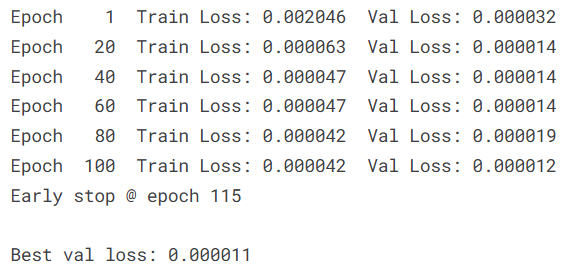AI Visual Insight: The image should show training logs or loss output, reflecting how the model gradually converges across epochs and how validation loss declines before stabilizing, indicating that optimization is working effectively.

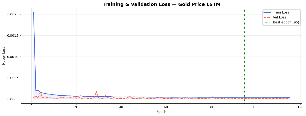AI Visual Insight: The image should contain training and validation loss curves, with the best epoch typically marked by a vertical line. This helps assess convergence speed, overfitting behavior, and whether learning rate scheduling is effective.

The test results are: MAE of 64.28 USD, RMSE of 100.89 USD, MAPE of 1.90%, and R² of 0.9859. For a long-horizon gold price series, these metrics indicate that the model can track the main trend with reasonable stability while keeping short-term deviations relatively low.

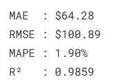AI Visual Insight: The image should show the evaluation metrics printed in the terminal, including MAE, RMSE, MAPE, and R². Together, these metrics describe error magnitude, relative error, and goodness of fit.

Visualization results show that the model is better at trend tracking than extreme-point prediction

The full-timeline prediction chart usually shows a close match between the predicted and actual lines, while a zoomed-in test-set view exposes deviations more clearly during periods of extreme volatility. This is a typical LSTM behavior in financial applications: strong on trend, weaker on spikes.

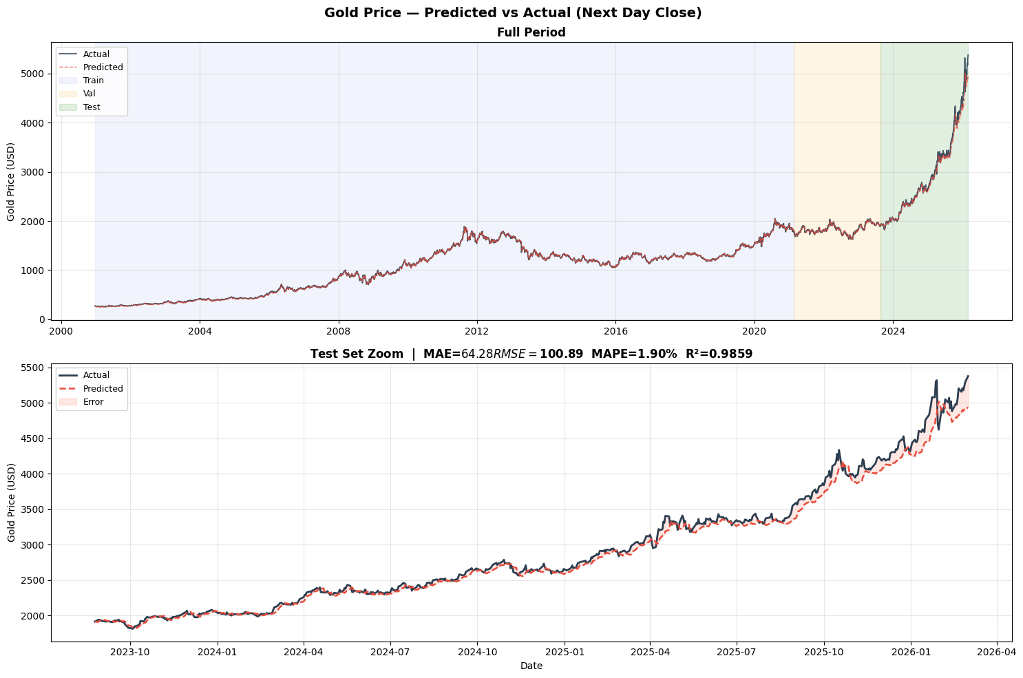AI Visual Insight: The image should include line plots of actual and predicted values across the full sample, shaded training/validation/test regions, and a zoomed test section, making it easy to inspect fit consistency and where errors are concentrated.

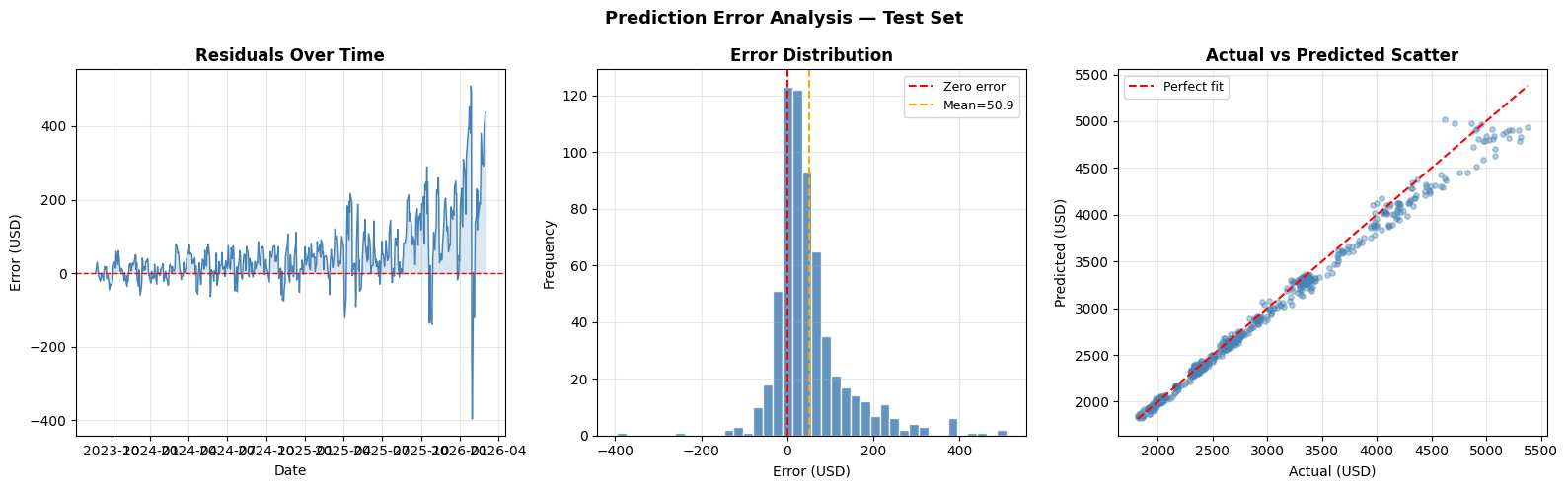AI Visual Insight: This image should be an error analysis panel, typically including a residual time series, an error histogram, and an actual-vs-predicted scatter plot. These views help identify systematic bias, whether the error distribution is symmetric, and whether the fit approaches the ideal diagonal line.

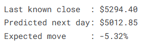
The final model can also be saved as gold_price_lstm.pt and used for next-day inference based on the most recent 30 days of data. This shows that the project is not just a teaching example, but also has a basic deployment-ready form.

AI Visual Insight: The image should show a final performance summary panel, including a bar chart of key metrics and a configuration table listing items such as window length, parameter count, optimizer, and loss function for quick experiment review.

The engineering value of this project lies in its complete time series forecasting template

From data cleaning, indicator construction, and sliding-window modeling to training control, error analysis, and model persistence, the workflow is complete and reusable. By replacing the data source and feature columns, the same template can be applied to crude oil, exchange rates, equities, or sales forecasting.

Further optimization directions include adding macroeconomic variables, holiday features, and multi-step forecasting tasks, as well as experimenting with BiLSTM, TCN, Transformer, or Attention-based hybrid architectures to improve robustness under extreme market conditions.

FAQ

Why doesn’t this project randomly shuffle the dataset?

Because time series data has a strict chronological order. Random shuffling leaks future information into the past and produces overly optimistic evaluation results. The correct approach is to split the training, validation, and test sets in time order.

Why add technical indicators such as moving averages, volatility, and momentum?

These indicators transform raw price changes into more interpretable features such as trend, dispersion, and deviation. They help the LSTM learn market structure faster instead of merely memorizing raw numeric values.

Can this model be used directly for live trading?

No. It should be treated as a research forecasting baseline rather than a production trading strategy. Before it can support live deployment, you need to incorporate transaction costs, slippage, risk controls, a backtesting framework, and macro-event shock handling.

Core Summary

This article reconstructs a PyTorch-based LSTM gold price forecasting project, covering data cleaning, technical indicator engineering, sliding-window modeling, training optimization, and error analysis. It includes key code snippets and chart interpretation, making it a practical template for financial time series forecasting.