This article focuses on UAV 3D path planning in complex mountainous environments. It proposes a unified optimization framework built on spherical-coordinate parameterization and a multi-objective cost function, then compares six algorithms—PSO, GWO, WOA, HHO, DBO, and SSA—across convergence speed, path smoothness, and safety. Keywords: UAV path planning, intelligent optimization algorithms, MATLAB.
Technical specifications are summarized below
| Parameter | Details |
|---|---|
| Primary Language | MATLAB |
| Application Scenario | UAV 3D path planning in mountainous terrain |
| Optimization Algorithms | PSO, GWO, WOA, HHO, DBO, SSA |
| Environment Model | Grid-based elevation terrain + cylindrical threat zones |
| Path Representation | Piecewise chained parameterization in spherical coordinates |
| Objective Function | Path length, threat avoidance, altitude safety, trajectory smoothness |
| Visualization Output | 3D terrain, top view, side view, convergence curves |
| Core Dependencies | MATLAB basic plotting and numerical computation toolboxes |
| Reference Popularity | The original article shows 50 reads |
This method addresses the high-dimensional planning bottleneck in complex 3D space
In complex mountainous environments, path planning is not simply about finding the shortest route. It is about balancing terrain variation, no-fly zones, flight altitude, and turning constraints. Traditional methods such as A*, Dijkstra, or RRT often produce redundant nodes, path jitter, and limited real-time performance in continuous 3D scenarios.
The key improvement in this approach is that it compresses a high-dimensional waypoint optimization problem into a low-dimensional parameter optimization problem. Instead of directly optimizing many 3D points, it optimizes the step length, elevation angle, and azimuth angle of each path segment, which significantly reduces the search space.
Spherical-coordinate parameterization makes path search better aligned with UAV motion
The chained spherical-coordinate model decomposes a path into multiple flight segments. Each segment requires only three parameters to recursively generate the next point in space. Compared with directly optimizing all waypoints in Cartesian coordinates, this representation is more compact and better matches how aircraft move in practice through heading and climb angle changes.
This representation provides three key advantages: lower optimization dimensionality, stronger physical interpretability, and easier constraint handling. It is especially effective when limiting climb angle and turning angle, where spherical coordinates are naturally more suitable than discrete point-based Cartesian representations.
function path = sph_path(startPoint, params)
% startPoint: Start coordinate [x,y,z]
% params: [step length, elevation angle, azimuth angle] for each segment
path = startPoint;                    % Initialize the path
current = startPoint;                 % Current point
for i = 1:size(params,1)
    r = params(i,1);                  % Step length of the current segment
    theta = params(i,2);              % Elevation angle
    phi = params(i,3);                % Azimuth angle
    dx = r * cos(theta) * cos(phi);   % Convert spherical coordinates to x increment
    dy = r * cos(theta) * sin(phi);   % Convert spherical coordinates to y increment
    dz = r * sin(theta);              % Convert spherical coordinates to z increment
    current = current + [dx, dy, dz]; % Recursively generate the next waypoint
    path = [path; current];           % Append to the path sequence
end
end
This code converts a low-dimensional spherical-parameter sequence into a complete 3D trajectory.
Environment modeling must represent both terrain and threat constraints
This approach abstracts real mountain terrain as a grid-based elevation field, where the X-Y plane indexes the corresponding ground elevation H. This allows the planner to quickly query the terrain altitude at any path point and determine whether the relative flight altitude is safe.
Threat zones are uniformly modeled as cylinders, which is a practical way to represent radar coverage, obstacles, and no-fly zones. Compared with irregular geometric models, cylindrical constraints are computationally cheaper and easier to couple with optimization algorithms.
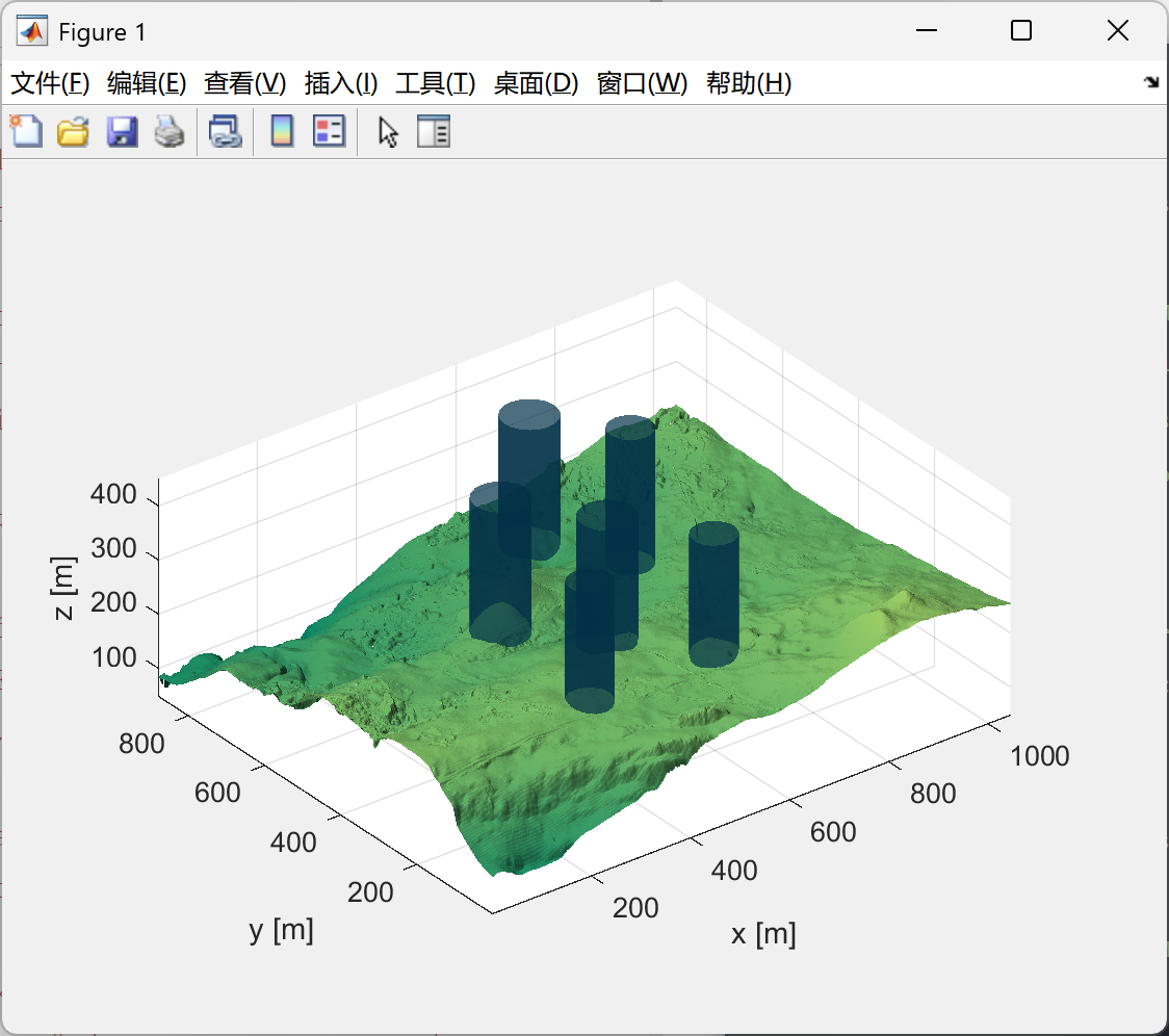 AI Visual Insight: This figure shows the overall spatial relationship between the 3D mountainous terrain and the planned flight path. The trajectory extends continuously above the undulating surface while actively avoiding raised terrain and threat zones, indicating that the model accounts for both terrain elevation and spatial obstacle-avoidance constraints. This view is mainly used to detect mountain collisions, obstacle penetration, or abrupt altitude changes.
The multi-objective cost function determines whether a path is actually flyable
This work does not optimize path length alone. Instead, it combines four cost components into a unified fitness function: path length, threat avoidance, altitude safety, and trajectory smoothness. As a result, the solution is not just short, but also safe, executable, and stable.
The threat cost uses hierarchical penalties, the altitude cost enforces valid clearance above the ground, and the smoothness cost limits abrupt turning and climb changes. This design is much closer to real flight-control requirements than using shortest path alone.
function J = cost_function(path, model, w)
L = calc_length(path);                 % Total path length cost
T = calc_threat_cost(path, model);     % Threat avoidance cost
H = calc_height_cost(path, model);     % Altitude safety cost
S = calc_smooth_cost(path);            % Trajectory smoothness cost
J = w(1)*L + w(2)*T + w(3)*H + w(4)*S; % Weighted total cost
end
This code transforms a multi-constraint planning problem into a single-objective problem that intelligent optimization algorithms can solve directly.
Comparing six intelligent optimization algorithms under one framework is more meaningful
This article evaluates PSO, GWO, WOA, HHO, DBO, and SSA under a unified environment, the same parameter scale, and the same evaluation metrics. This point matters because many comparison studies become distorted when initialization conditions differ.
PSO has a simple structure and converges quickly, but it tends to get trapped in premature convergence in complex non-convex spaces. GWO and WOA are more stable in global exploration, but their late-stage fine search ability is limited in highly constrained 3D environments.
Newer swarm intelligence algorithms usually perform better in complex scenarios
HHO, DBO, and SSA share a common strength: they offer more flexible exploration and exploitation mechanisms. Through more sophisticated population role assignment or hunting strategies, they are more likely to find low-cost solutions in scenarios that must balance obstacle avoidance, climb behavior, and smoothness.
The conclusion from the source material is also clear: HHO, DBO, and SSA outperform PSO, GWO, and WOA overall in convergence speed, robustness, and final path quality, especially in complex mountainous terrain with dense threats.
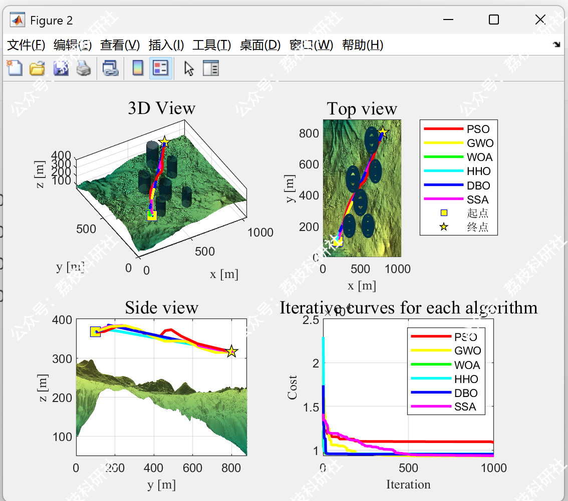 AI Visual Insight: This figure emphasizes obstacle avoidance from a planar or local perspective, making it easier to inspect the trajectory offset from threat boundaries and the continuity of direction changes. If the path contains dense polylines or sharp turns near obstacle edges, the smoothness cost weight is usually too low. If the detour distance is excessive, the threat penalty weight is likely too high.
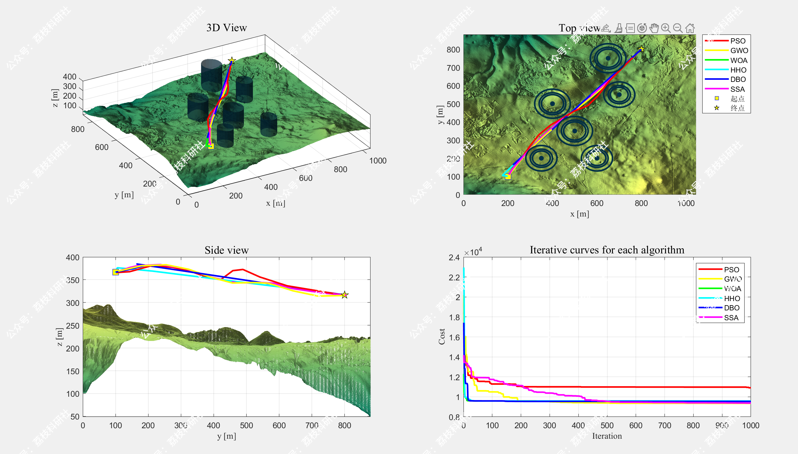 AI Visual Insight: This figure presents altitude variation or an aggregated result from another viewpoint, making it suitable for checking whether the trajectory stays within a safe flight envelope. If the path closely follows terrain fluctuations, the algorithm is likely prioritizing shorter distance. If altitude changes are too aggressive, energy consumption and control difficulty may increase.
The MATLAB visualization code reflects the result-validation pipeline
The original article includes a PlotModel function for rendering 3D terrain and cylindrical threat zones, which forms the basis of experimental interpretability. It does more than mesh rendering. It also improves spatial readability through lighting, transparency, and material settings.
The equivalent implementation below is organized for quick understanding of its core logic.
function PlotModel(model)
mesh(model.X, model.Y, model.H);                 % Draw the 3D terrain mesh
colormap(summer);                                % Use the summer colormap to represent elevation
shading interp;                                  % Smooth shading for better readability
axis equal; hold on;                             % Preserve scale and overlay plots

threats = model.threats;                         % Load threat-zone parameters
h = 250;                                         % Set the cylinder threat height
for i = 1:size(threats, 1)
    threat = threats(i,:);                       % Current threat [x,y,z,r]
    [xc, yc, zc] = cylinder(threat(4));          % Generate a cylinder from the radius
    xc = xc + threat(1);                         % Translate to the threat center in x
    yc = yc + threat(2);                         % Translate to the threat center in y
    zc = zc * h + threat(3);                     % Scale and translate the z height
    c = mesh(xc, yc, zc);                        % Draw the cylindrical threat zone
    set(c, 'edgecolor', 'none', ...
        'facecolor', [2 48 71]/255, ...          % Set the threat-zone color
        'FaceAlpha', 0.7);                       % Set transparency for easier path inspection
end
end
This code visualizes the terrain field and threat zones in 3D, providing an intuitive basis for path-feasibility verification.
The engineering value of this study lies in transferability and scalability
The real value of this method is not a single simulation result, but the transferable technical framework it establishes: environment modeling, parameterized representation, a unified cost function, unified algorithm testing, and unified visualization output across the full workflow.
From an engineering perspective, it applies to inspection, search and rescue, border patrol, and military reconnaissance tasks that require low-altitude autonomous navigation. If future work integrates energy-consumption models, communication links, dynamic obstacles, or online replanning mechanisms, the system can move much closer to real-world deployment.
FAQ: The three questions developers care about most
Q1: Why is spherical-coordinate parameterization more suitable than directly optimizing 3D waypoints for this problem?
A1: Because spherical coordinates describe the trajectory with step length, elevation angle, and azimuth angle, they use fewer variables and support more natural constraints. This significantly reduces dimensionality and improves convergence efficiency.
Q2: Which algorithms should I try first among the six?
A2: If your goal is high-quality paths in complex mountainous terrain, start with HHO, DBO, and SSA. If you need a fast baseline model, begin with PSO or GWO.
Q3: Can this MATLAB framework be directly migrated to Python or ROS?
A3: Yes. The core ideas are the environment representation, parameterization strategy, and cost-function design. All of these can be migrated to NumPy, PyTorch, or ROS/Gazebo, while MATLAB mainly serves for prototyping and visualization.
Core summary
This article reconstructs a UAV 3D path planning solution for complex mountainous environments. Its core ideas are chained spherical-coordinate parameterization and a multi-objective cost function. Under a unified MATLAB framework, it performs a side-by-side comparison of PSO, GWO, WOA, HHO, DBO, and SSA, and provides conclusions on modeling, optimization, visualization, and engineering applicability.