This article is written for participants in the 2026 May Day Mathematical Modeling Contest. It distills the core tasks, difficulty levels, and modeling routes of Problem A on coal mine support, Problem B on flexible scheduling, and Problem C on slope early warning, helping teams choose a topic within 5 to 10 minutes. Keywords: mathematical modeling, topic selection analysis, optimization, forecasting.
Technical Specification Snapshot
| Parameter | Details |
|---|---|
| Domain | Mathematical modeling contest topic analysis |
| Primary Languages | Python / MATLAB |
| Problem Types | Parameter fitting, scheduling optimization, time-series forecasting |
| Common Algorithms | Regression, MILP, Genetic Algorithm, LSTM, changepoint detection |
| Data Types | Experimental data, process constraints, multi-source time-series monitoring data |
| Original Popularity | Approximately 288 views |
| Core Dependencies | pandas, numpy, scikit-learn, pulp, xgboost, ruptures |
Problem C is the safest choice overall, Problem B comes next, and Problem A is more mechanism-driven.
The original analysis presents a clear topic preference: the estimated participant distribution is A:B:C = 1:2:3, and the estimated difficulty is A:B:C = 5:4:3. If you evaluate topics by a combined metric of “probability of winning + speed of execution,” Problem C is the best fit for most teams, Problem B suits teams with strong optimization skills, and Problem A is better for participants with mechanics or geotechnical backgrounds.
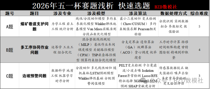 AI Visual Insight: This image is an overview infographic of the contest problems. Its main value is that it compresses the expected participant volume, difficulty level, and problem structure of Problems A, B, and C into a single visual panel. It works well as a rapid decision aid at the beginning of the competition, helping teams build a global understanding of the topics in very little time.
From a competition strategy perspective, the best topic is not simply the “easiest” one. It is the one that can reliably produce a solid paper structure. Problem C naturally includes data cleaning, stage identification, prediction, and early warning, so its paper skeleton is inherently complete. Problem B has a standard optimization framework, which makes it easy to write a layered model design. Problem A has a clear problem chain, but it demands stronger mechanistic interpretation and more credible parameter justification.
A practical scoring framework for topic selection
scores = {
    "A": {"difficulty": 5, "data_cleanliness": 3, "innovation_space": 4},
    "B": {"difficulty": 4, "data_cleanliness": 4, "innovation_space": 5},
    "C": {"difficulty": 3, "data_cleanliness": 3, "innovation_space": 5}
}

# Score each topic using low difficulty, high innovation, and strong write-up potential
for topic, v in scores.items():
    total = (6 - v["difficulty"]) * 0.4 + v["innovation_space"] * 0.4 + v["data_cleanliness"] * 0.2  # Core scoring logic
    print(topic, round(total, 2))  # Output the overall topic score
This code converts subjective topic selection experience into comparable quantitative scores.
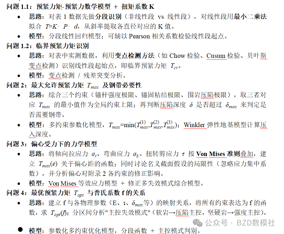
Problem A is fundamentally a nonlinear support mechanism model with multi-constraint optimization.
Problem A focuses on bolt support in coal mine roadways. The core variable is the relationship between pre-tightening torque T and pre-tightening force P. The main challenge is that this mapping is not a single linear relationship. It is affected by thread clearance, contact friction, and surrounding rock conditions, producing piecewise nonlinear behavior.
 AI Visual Insight: This figure shows the structural schematic of the coal mine bolt support problem. It typically includes load-bearing components, pre-tightening application points, and key geometric parameters. For modeling, the value of this type of image lies in helping identify the torque-to-axial-force transmission path, eccentricity effects, and the sources of discrepancy between field conditions and experimental conditions.
A practical modeling route has three steps: first fit the T-P parameters, then introduce corrections for eccentric distance and surrounding rock differences, and finally perform multi-objective or multi-constraint optimization. If the dataset is limited, piecewise regression is usually more stable than a complex neural network. If you want more innovation, you can add Gaussian Process Regression or Support Vector Regression.
A minimum viable modeling pipeline for Problem A
import numpy as np
from sklearn.preprocessing import PolynomialFeatures
from sklearn.linear_model import LinearRegression

T = np.array([10, 20, 30, 40]).reshape(-1, 1)
P = np.array([15, 33, 52, 70])

poly = PolynomialFeatures(degree=2, include_bias=False)
T2 = poly.fit_transform(T)  # Expand torque into quadratic features
model = LinearRegression()
model.fit(T2, P)  # Fit the nonlinear T-P relationship
pred = model.predict(T2)
This code demonstrates the most common starting point for nonlinear fitting in Problem A.
Problem B allows teams with operations research strengths to build a high-quality paper quickly.
Problem B is essentially a Flexible Job Shop Scheduling Problem, with additional layers such as inter-workshop transfer, dual-crew coordination, and budget constraints. Its advantage is that the problem structure is standard and the terminology is mature, so it maps easily to existing frameworks such as MILP, Genetic Algorithms, and Ant Colony Optimization.
Problems 1 through 4 form a stepwise progression: start with single-workshop scheduling, then move to joint optimization of multi-workshop routing and scheduling, then add crew coordination, and finally solve the integrated decision problem of equipment procurement and scheduling. For paper organization, this progressive structure is highly friendly.
The main modeling line for Problem B should start with exact models and then extend with heuristics.
jobs = ["J1", "J2", "J3"]
machines = ["M1", "M2"]
process_time = {("J1", "M1"): 3, ("J2", "M2"): 4, ("J3", "M1"): 2}

schedule = []
current_time = {"M1": 0, "M2": 0}

for job, machine in [("J1", "M1"), ("J2", "M2"), ("J3", "M1")]:
    start = current_time[machine]
    end = start + process_time[(job, machine)]  # Compute the completion time of this operation
    schedule.append((job, machine, start, end))
    current_time[machine] = end  # Update the machine occupancy window
This code shows the most basic time-window propagation logic in scheduling problems.
If the team is short on time, use integer programming to build the baseline model for Problems 1 and 2, then add a Genetic Algorithm or NSGA-II for Problems 3 and 4 as an extension. This preserves rigor while also creating a paper highlight with an “exact method + heuristic method” structure.
Problem C offers the most complete data science loop, so it delivers the best overall value.
Problem C is set in the context of slope early warning and covers data correction, changepoint detection, anomaly identification, multivariate forecasting, and warning-threshold design. Its strengths are a complete workflow, strong algorithm substitutability, rich visualization space, and naturally abundant innovation points.
More specifically, Problem 1 is correction, Problem 2 is stage identification, Problem 3 is cleaning and correlation analysis, Problem 4 is prediction, and Problem 5 is variable selection and early warning. This task chain is very close to a real industrial monitoring system, so the resulting paper is less likely to feel superficial.
The most important breakthrough for Problem C is stage-wise modeling.
import ruptures as rpt
import numpy as np

signal = np.array([1, 2, 3, 3, 4, 8, 9, 10, 10, 11])
model = rpt.Pelt(model="rbf").fit(signal)
bkps = model.predict(pen=2)  # Identify stage transition points
print(bkps)
This code identifies changepoints in a displacement sequence and serves as a key entry point for Question 2 of Problem C.
You can then model each stage separately: use linear regression in the early stage, XGBoost in the middle stage, and LSTM or Transformer models in the pre-failure stage. This approach aligns with the mechanism of three-stage deformation and significantly improves interpretability.
Practical topic selection should be based on team capability rather than topic popularity.
If your team is stronger in data analysis and machine learning, choose Problem C first. If your team is stronger in operations research, integer programming, and algorithm design, choose Problem B first. If your members have geotechnical, mechanics, or engineering backgrounds, Problem A may actually create a differentiation advantage.
More importantly, do not turn innovation into a mere “list of algorithms.” Judges care more about whether the problem decomposition is clear, whether the evaluation metrics are verifiable, and whether the results are well explained. In contests like the May Day Cup, steady completion matters more than showing off technical complexity.
FAQ
1. Which problem is best for finishing a high-quality paper within three days?
Problem C is the best choice. Its data-processing chain is naturally complete, making it easy to form a standard paper structure of “cleaning → analysis → prediction → early warning.”
2. Does Problem B require a Genetic Algorithm or Reinforcement Learning?
Not necessarily. It is usually more stable to build an interpretable baseline model with MILP first, then use a Genetic Algorithm as an extension. This often scores better than jumping directly to a complex intelligent algorithm.
3. Is the main difficulty in Problem A the formula or the data?
The core difficulty lies in mechanistic interpretation and parameter explanation. Even if the fitting performance looks good, the paper remains unconvincing if it cannot explain why friction, eccentricity, and surrounding rock differences affect the T-P relationship.
AI Readability Summary
This article reconstructs the core tasks, modeling routes, and topic selection recommendations for Problems A, B, and C in the 2026 23rd May Day Mathematical Modeling Contest, helping teams make a fast and informed decision. It focuses on three problem types—coal mine support, flexible job shop scheduling, and slope early warning—and provides algorithm stacks, innovation directions, and fast project-start strategies.