This project builds a car sales analysis system around Dongchedi sales data. Its core capabilities include multi-brand data collection, structured storage, Django-based visualization, and sales forecasting. It solves the problem of fragmented, hard-to-track, and hard-to-compare automotive sales data. Keywords: Python web scraping, Django, ECharts.
Technical specifications provide a quick implementation snapshot
| Parameter | Description |
|---|---|
| Programming Language | Python |
| Web Framework | Django |
| Database | MySQL |
| Visualization | ECharts |
| Data Source Protocol | HTTP/HTTPS requests |
| Target Brands | NIO, Li Auto, XPeng, Xiaomi Auto, Zeekr |
| Star Count | Not provided in the source |
| Core Dependencies | requests, Django ORM, PyMySQL, ECharts, tqdm |
The system covers the full pipeline from collection to analysis
This project is not just a single chart page. It implements a complete data pipeline: scrape monthly sales data from Dongchedi, write it into MySQL, import it into Django models, and finally generate multi-dimensional analysis pages.
Its value lies in turning fragmented web data into a business asset that is queryable, comparable, and predictable. That makes it well suited for course projects, data analysis practice, and visualization demos.
The directory structure reflects clear module boundaries
懂车帝汽车销售数据分析/
├── spider/
│   ├── scraw.py
│   ├── import_data.py
│   └── sales_vehicledata.csv
├── myapp/
│   ├── models.py
│   └── views.py
├── templates/
│   ├── VehicleSales.html
│   ├── VehicleSalesTrend.html
│   ├── VehiclePriceSales.html
│   ├── ChampionVehicles.html
│   └── VehicleSalesPrediction.html
└── static/
This layout defines a three-layer structure for collection, import, and presentation, making it easier to replace data sources or add new pages later.
The scraper module collects monthly sales through parameterized requests
The scraper operates across two dimensions: brand and month. It supports continuous backward collection from a specified starting month and incremental updates for the current month, which makes it suitable for building a long-term sales dataset.
The original implementation emphasizes rate limiting, retry handling, and multi-brand collection. That means the system is not a one-off script, but a reusable data pipeline.
Request parameter construction determines collection scalability
def build_rank_params(month, brand_id):
    return {
        "aid": "1839",
        "app_name": "auto_web_pc",
        "count": "100",
        "offset": "0",
        "month": "" if month in (None, "") else str(month),  # Fetch historical ranking data by month
        "rank_data_type": "11",
        "brand_id": str(brand_id),  # Collect data for a specific brand ID
        "nation": "0",
    }
This function generates a unified parameter set for brand sales ranking requests, making batch scheduling and reuse much easier.
Replace-style writes preserve monthly data consistency
def replace_month_sales(conn, month, sales_list):
    rows = transform_sales_rows(month, sales_list)  # Convert the raw response into database rows first
    with conn.cursor() as cursor:
        cursor.execute("DELETE FROM sales_vehicledata WHERE month = %s", (month,))
        if rows:
            cursor.executemany(
                "INSERT INTO sales_vehicledata (...) VALUES (...) ON DUPLICATE KEY UPDATE ...",
                rows,
            )
    conn.commit()  # Commit the transaction to make this month's data effective as a whole
    return len(rows)
This logic uses a delete-then-insert pattern plus conflict updates to ensure that data for the same month does not accumulate in duplicate.
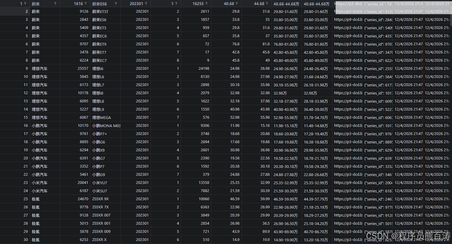 AI Visual Insight: This image shows the database write results after the scraping script runs. It typically includes monthly batches, the number of records written per brand, and database status, which helps verify whether parallel multi-brand collection, historical backfill, and incremental updates executed successfully.
The data import module aligns CSV files with the Django ORM
If collected results are first stored in CSV format, the system also provides an import script to sync structured files into Django models. This step works well for local development, offline demos, and data repair.
Its core value is not simple insertion. Instead, it performs idempotent updates based on series_id + month, which prevents duplicate imports from creating dirty data.
update_or_create makes the import process idempotent
def import_data(reader):
    created_count, updated_count = 0, 0
    for row in reader:
        obj, created = VehicleData.objects.update_or_create(
            series_id=int(row["series_id"]),
            month=int(row["month"]),  # Series and month together define a unique record
            defaults={
                "brand_name": row["brand_name"],
                "series_name": row["series_name"],
                "sales_count": int(row["sales_count"]),
            },
        )
        if created:
            created_count += 1
        else:
            updated_count += 1
This function safely imports CSV data into Django and automatically distinguishes between inserts and updates.
The visualization module turns sales data into decision-ready views
The frontend analytics section is the most presentation-friendly part of the project. It covers total brand sales, vehicle series trends, price ranges, champion rankings, and future forecasts, forming an analysis chain of describing the current state, explaining relationships, and projecting the future.
These pages share the Django view layer and ORM aggregation logic, so the cost of extending them remains low.
The sales overview page compares total volume across brands and series
The /vehicle-sales/ page uses annotate(Sum('sales_count')) to aggregate sales by brand and series. It is ideal for understanding overall scale first and then drilling down into the internal structure of a brand.
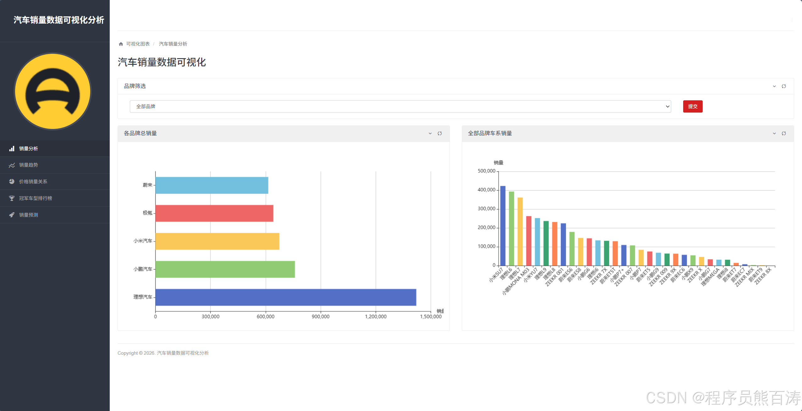 AI Visual Insight: This page typically includes a bar chart for total brand sales and a linked series list area. It clearly shows the sales gap among brands such as Li Auto, NIO, and XPeng, as well as the contribution share of core models within a brand.
The sales trend page identifies cyclical changes and breakout model volatility
The /vehicle-trend/ page filters by year and brand, then maps each vehicle series into a 12-month sales sequence. It is useful for identifying new product launches, seasonal fluctuations, and the staying power of top-selling models.
def build_series_data(all_data, year_int):
    series_dict = {}
    for item in all_data:
        name = item["series_name"]
        month = item["month"]
        sales = item["sales_count"]
        series_dict.setdefault(name, {})
        series_dict[name][month] = series_dict[name].get(month, 0) + sales  # Accumulate and deduplicate same-month data
    return series_dict
This function organizes discrete query results into a time-series structure that line charts can consume directly.
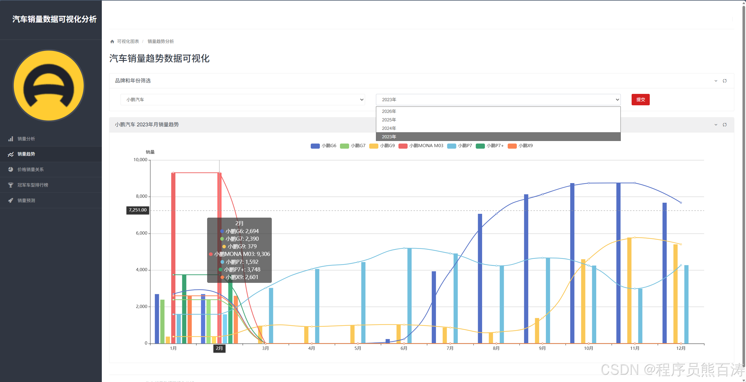 AI Visual Insight: This chart typically overlays multiple vehicle series lines and highlights the month axis, sales axis, and brand filter interactions. It is useful for observing whether certain models show sustained growth, short-term spikes, or seasonal declines.
The price-to-sales page reveals market segmentation
The /price-sales/ page combines scatter plots, range-based bar charts, average trend lines, and box plots. It answers not only which vehicles sell well, but also which price bands are more likely to achieve scaled sales.
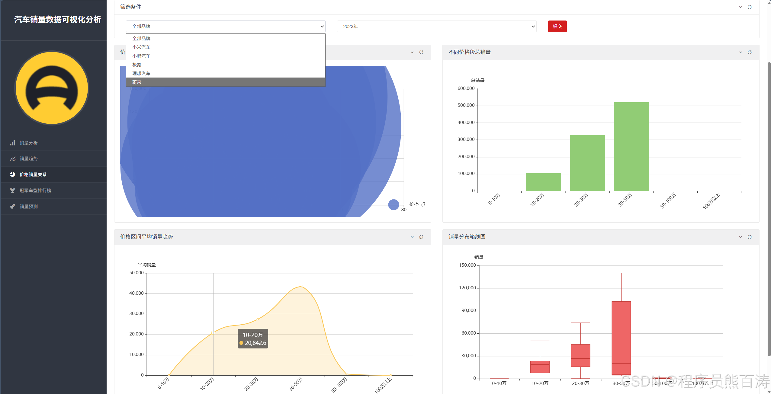 AI Visual Insight: This page typically uses scatter points to map price to sales for individual models, while bar charts and box plots summarize the distribution of price bands. It helps identify sales concentration and dispersion in core market segments such as 100k–200k RMB and 200k–300k RMB.
Champion model and sales forecast pages add interpretability and forward-looking value
The champion ranking page focuses on which model wins first place most often, while the forecasting page focuses on which models are likely to keep leading in the next stage. Together, they upgrade the system from a static query interface to a lightweight analytics platform.
The champion model page extracts the competitive landscape of monthly winners
The /champion-vehicles/ page filters with rank_no=1 to extract the monthly champion, then renders a heatmap, a bar chart of champion counts, and a pie chart of brand share.
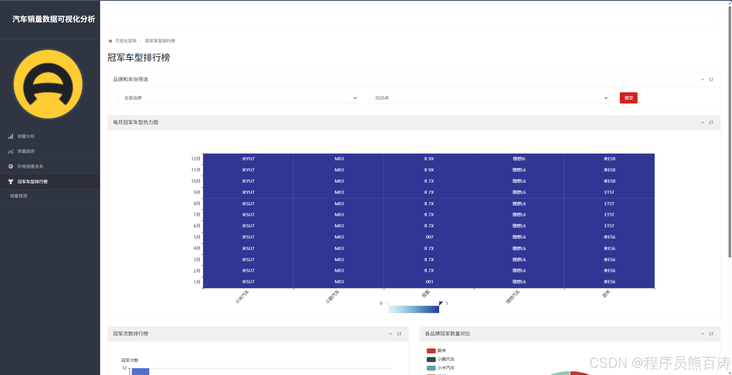 AI Visual Insight: This chart uses brand and month as two-dimensional coordinates and marks champion models with colored cells or labels. It helps reveal whether a brand dominates the year with one long-running bestseller or switches its best-selling model across different months.
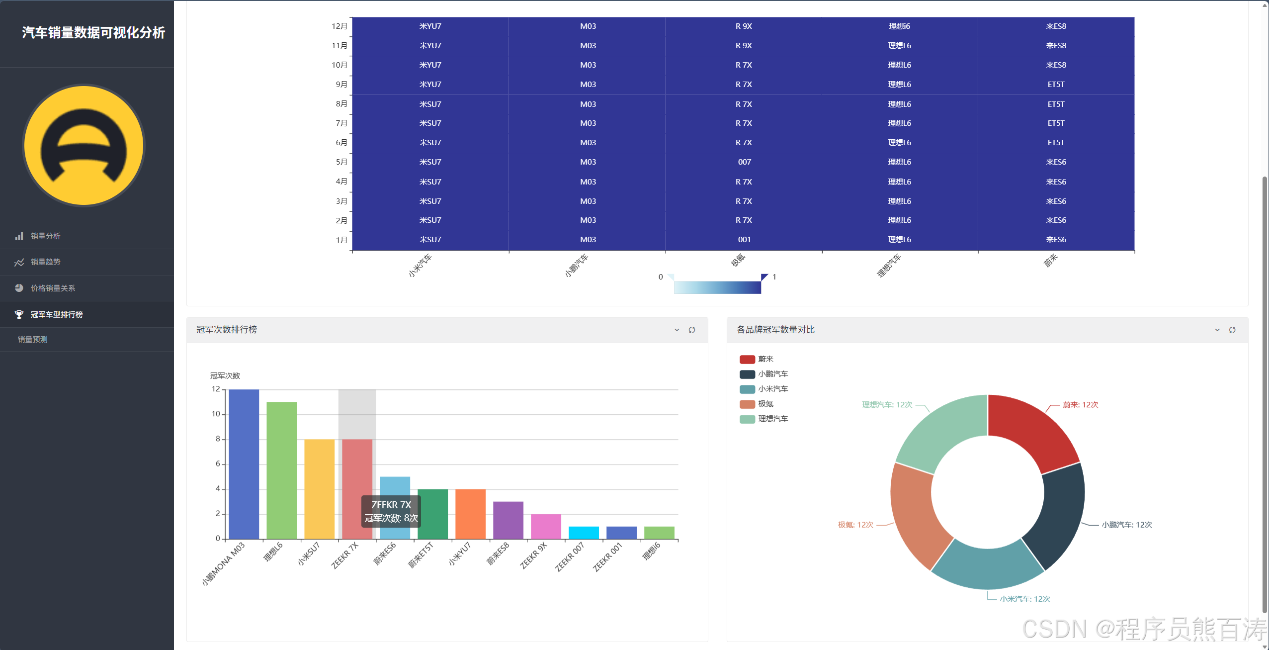 AI Visual Insight: This view typically places champion count rankings for vehicle series alongside brand-level champion share. It lets you compare whether the strongest single model and the strongest overall brand are actually the same, revealing the difference between brand breadth and blockbuster depth.
The sales forecast page uses a composite algorithm to reduce single-model bias
This page combines four methods: MA-3, WMA, ETS, and linear trend, then computes a weighted average across them. It is not a strict machine learning approach, but it is more robust when the dataset is limited.
def predict_sales(recent_sales):
    predictions = []
    ma3 = sum(recent_sales[-3:]) / 3
    predictions.append((ma3, 0.2))  # Simple average of the most recent three months
    wma = recent_sales[-3] * 0.2 + recent_sales[-2] * 0.3 + recent_sales[-1] * 0.5
    predictions.append((wma, 0.25))  # Give more weight to more recent data
    final_pred = sum(p * w for p, w in predictions) / sum(w for p, w in predictions)
    return final_pred
This function blends multiple time-series estimation methods to produce a smoother future sales forecast.
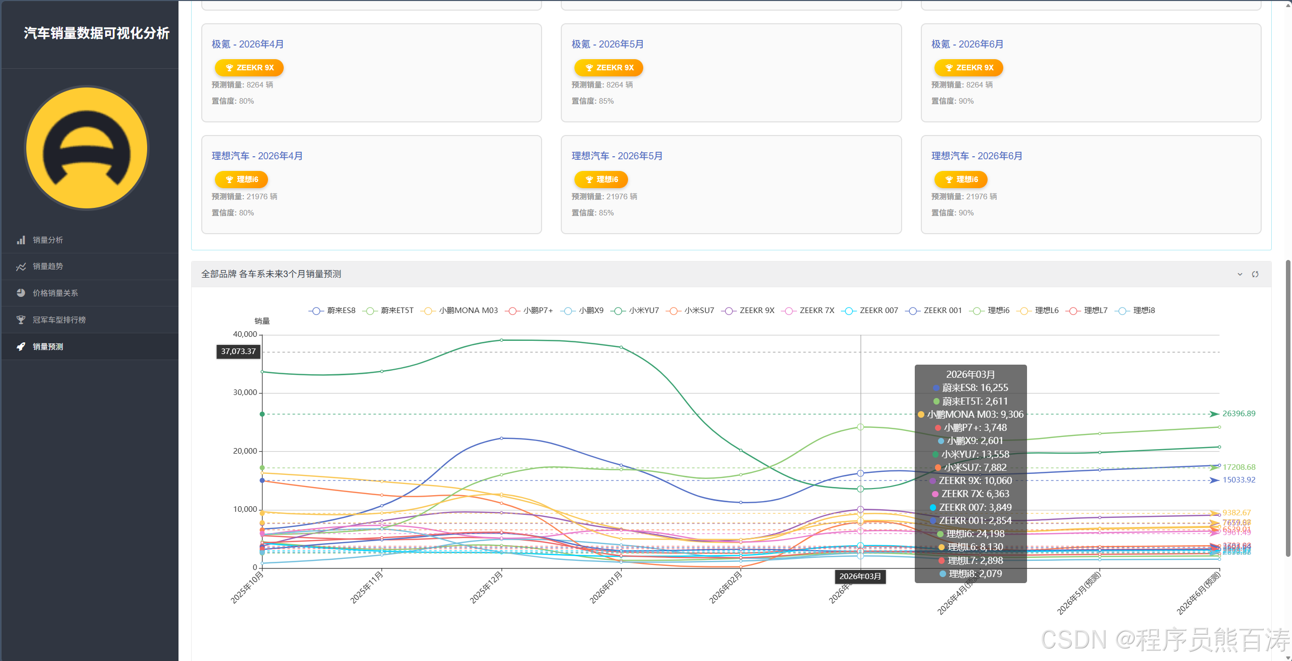
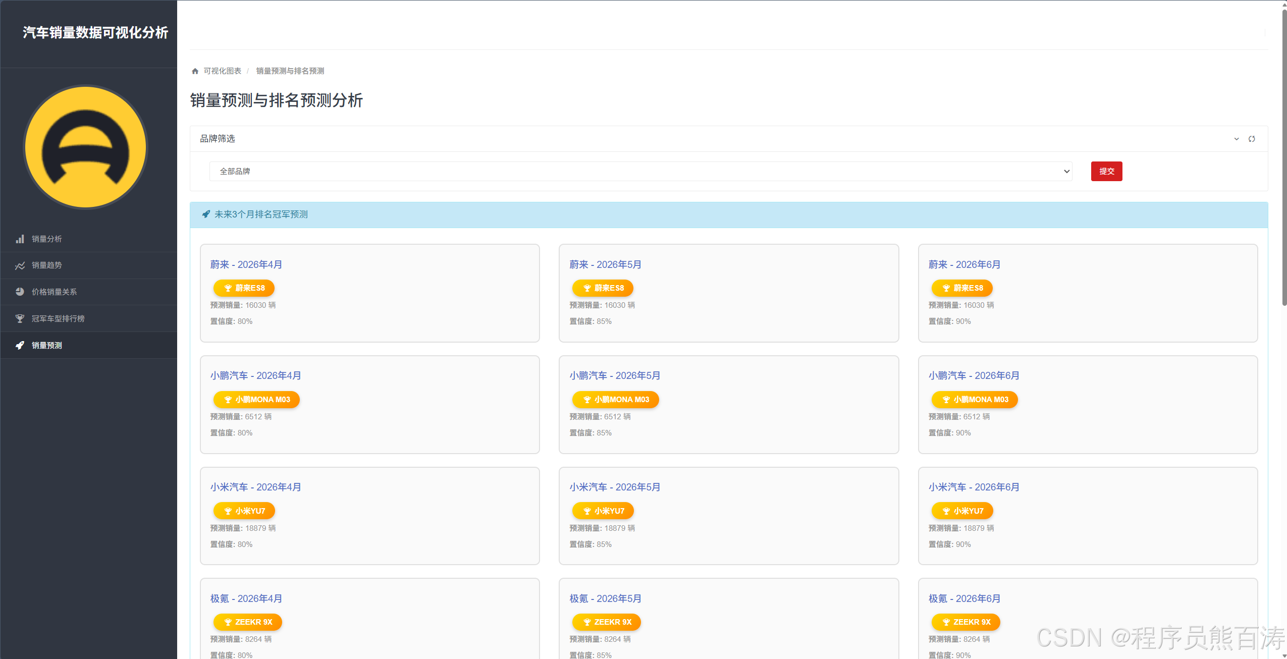 AI Visual Insight: This page typically includes a historical sales line chart, a three-month forecast line, and champion forecast cards. It emphasizes trend continuity, inflection points, and the potential leading models for each brand.
 AI Visual Insight: This image is more explanatory in nature. It often shows algorithm weights, forecast values, and confidence explanation areas, helping users understand that the result is not a black box but a combination of multiple statistical methods.
This project works well as both a teaching case and a business prototype
From an engineering perspective, it already includes the key stages of collection, cleaning, storage, aggregation, charting, and forecasting. For academic course work, it is complete enough. For enterprise prototyping, it can serve as the foundation of a new energy vehicle sales analytics backend.
If you continue enhancing it, consider adding a scheduler, anomaly monitoring, API encapsulation, and more formal time-series models such as Prophet, XGBoost, or LSTM.
FAQ
1. Why does this system use Django instead of a fully separated frontend and backend architecture?
Django includes ORM, templates, routing, and admin capabilities out of the box, which makes it a strong fit for rapidly building data analysis projects. For small to medium demo systems, development efficiency is usually higher than with a fully separated architecture.
2. Why do both the import and collection stages use updates instead of append-only writes?
Sales rankings may be revised over time, and repeated appends can create conflicts for the same month and vehicle series. Using DELETE + INSERT or update_or_create ensures that the latest data always remains the source of truth.
3. What is the value of the composite forecasting algorithm?
A single forecasting method can be heavily affected by short-term fluctuations. Combining MA, WMA, ETS, and trend regression improves stability when the sample size is small, making it more suitable for teaching projects and lightweight business forecasting.
AI Readability Summary: This article reconstructs a car sales data analytics system for new energy vehicle brands. It covers Dongchedi data collection, MySQL storage, Django import workflows, and ECharts-based visualization, while explaining the core implementation behind sales trends, price segmentation, champion models, and composite forecasting.