EfficientNetB5 Poultry Disease Image Classification: A Practical Guide to High-Accuracy Chicken Disease Detection - Devuly | Smart Analytics for Developers & Projects

This project uses the Kaggle poultry disease image dataset to build a chicken disease classification model with EfficientNetB5. It identifies four classes—Coccidiosis, Healthy, Newcastle Disease, and Salmonella—to address the challenges of early diagnosis in remote farms where veterinary resources are limited. Keywords: EfficientNetB5, transfer learning, image classification.

Table of Contents

This project builds a low-cost chicken disease recognition solution for real farming scenarios

Parameter	Details
Primary Language	Python 3.9
Deep Learning Framework	TensorFlow / Keras
Image Processing	OpenCV, Matplotlib
Data Processing	Pandas, NumPy, scikit-learn
Model Architecture	EfficientNetB5
Input Size	180×180 or 224×224
Classification Classes	Coccidiosis, Healthy, Newcastle Disease, Salmonella
Data Source	Kaggle Poultry Disease Diagnosis Dataset
License	Source content marked as CC 4.0 BY-SA
Star Count	Not provided in the original source
Core Dependencies	tensorflow, opencv-python, scikit-learn, pandas

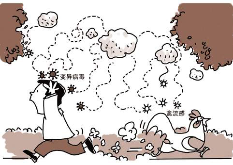AI Visual Insight: The image presents the project’s application scenario. The central focus is poultry disease recognition based on fecal images, highlighting the combination of field sampling, visual diagnosis, and intelligent farming.

This dataset provides real-world collection conditions and a clear four-class objective

The dataset was collected in the Arusha and Kilimanjaro regions of Tanzania, and samples were captured through the ODK tool on mobile phones. These are not laboratory images with clean white backgrounds. Instead, they come from real-world environments with complex background noise, which means the model must be more robust.

The dataset contains four labels: Coccidiosis, Healthy, New Castle Disease, and Salmonella. The original source also notes that images were resized to 224×224, which aligns well with the input requirements of transfer learning models.

Data loading first solves path management and label structuring

import pandas as pd

# Read the image path and label mapping table
csvpath = '/kaggle/input/chicken-disease-1/train_data.csv'
df = pd.read_csv(csvpath)

# Standardize column names for downstream processing
df.columns = ['filepaths', 'labels']
print(df.head())  # Check whether sample paths and labels loaded correctly

This code reads and structures the training metadata, which serves as the entry point for later image preprocessing and label encoding.

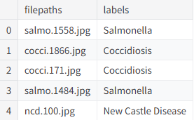AI Visual Insight: The image appears to show a DataFrame preview with filepaths and labels columns, confirming that sample indices, image paths, and disease labels were aligned successfully.

Sample visualization can reveal labeling and quality issues early

In image classification, inspecting the data before training is a hard rule. This project uses Matplotlib to display the first nine samples and checks whether images are corrupted, whether labels are mismatched, and whether pathological features appear learnable.

AI Visual Insight: The image shows a 3×3 sample grid, where different subplots correspond to different disease classes. The backgrounds are not consistent, which indicates that the model must extract stable pathological texture features from complex environments.

import cv2
import matplotlib.pyplot as plt

fig, ax = plt.subplots(3, 3, figsize=(12, 12))
ax = ax.ravel()

for idx in range(min(9, len(df))):
    img = cv2.imread(df['filepaths'][idx])
    if img is not None:
        img = cv2.resize(img, (224, 224))  # Standardize the input size
        img = cv2.cvtColor(img, cv2.COLOR_BGR2RGB)  # Convert BGR to RGB
        ax[idx].imshow(img)
        ax[idx].set_title(df['labels'][idx])
        ax[idx].axis('off')
plt.tight_layout()
plt.show()

This code provides a fast sample inspection step and helps prevent invalid data from entering the training pipeline.

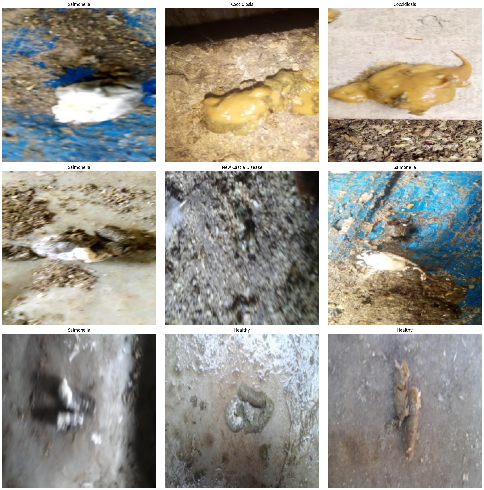AI Visual Insight: The image likely shows the visualization output with multiple labeled poultry fecal samples. Different classes exhibit fine-grained differences in color, texture, and shape, which are the discriminative cues the convolutional network must learn.

Feature engineering converts raw images into trainable tensors

This project defines a transform_data function to resize and normalize images and encode text labels into one-hot vectors. The original source contains a small bug: it prints shapes using undefined variables X_train and y_train, so the variable names should remain consistent in practice.

import numpy as np
from sklearn.preprocessing import LabelEncoder
from tensorflow.keras.utils import to_categorical

def transform_data(df, image_size=(180, 180)):
    images, labels = [], []
    for _, row in df.iterrows():
        img = cv2.imread(row['filepaths'])
        if img is not None:
            img = cv2.resize(img, image_size)  # Standardize the model input resolution
            img = img / 255.0  # Normalize to the 0-1 range
            images.append(img)
            labels.append(row['labels'])

    X = np.array(images)
    lb = LabelEncoder()
    y = lb.fit_transform(labels)
    y = to_categorical(y, num_classes=4)  # Convert to four-class one-hot labels
    return X, y, lb

This code completes image tensor conversion and label numerical encoding, which is a critical standardization step before transfer learning training.

AI Visual Insight: The image shows the shape outputs of the preprocessed data, typically including sample count, image height and width, channel count, and label dimensions. This helps confirm that the input tensors and classification targets are aligned.

Stratified splitting keeps class distributions consistent across train and test sets

The project uses a two-stage split strategy to produce 80% training, 10% validation, and 10% test subsets. It also enables stratify to reduce evaluation bias caused by class imbalance.

from sklearn.model_selection import train_test_split

X_train, X_temp, y_train, y_temp = train_test_split(
    X, y, train_size=0.8, random_state=123, shuffle=True, stratify=y
)
X_val, X_test, y_val, y_test = train_test_split(
    X_temp, y_temp, test_size=0.5, random_state=123, shuffle=True, stratify=y_temp
)

This code keeps the training, validation, and test subsets as statistically consistent as possible.

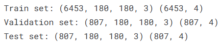AI Visual Insight: The image likely shows the shapes of the three dataset splits, confirming that each subset has a clear size and is suitable for training monitoring and independent test evaluation.

EfficientNetB5 transfer learning is the main source of accuracy in this solution

The original project uses EfficientNetB5 as the feature extraction backbone and adds several fully connected layers for four-class classification. Its advantages include strong parameter efficiency and expressive feature learning, making it well suited to medium- and high-accuracy agricultural vision tasks.

Two implementation details deserve attention. First, the original source uses both ImageDataGenerator and manual normalization, which creates a risk of duplicate scaling. Second, it calls compile twice, while only one call is actually necessary.

from tensorflow.keras.applications import EfficientNetB5
from tensorflow.keras.models import Sequential
from tensorflow.keras.layers import Flatten, Dense, BatchNormalization
from tensorflow.keras.optimizers import Adam

base_model = EfficientNetB5(
    weights='imagenet', include_top=False, input_shape=(180, 180, 3)
)
base_model.trainable = True  # Enable fine-tuning for agricultural disease image features

model = Sequential([
    base_model,
    Flatten(),
    Dense(256, activation='relu'),
    BatchNormalization(),
    Dense(128, activation='relu'),
    Dense(64, activation='relu'),
    Dense(4, activation='softmax')  # Output probabilities for four classes
])

model.compile(
    optimizer=Adam(learning_rate=1e-4),
    loss='categorical_crossentropy',
    metrics=['accuracy']
)

This code defines the complete classifier, with the core idea of transfer learning from ImageNet-pretrained weights.

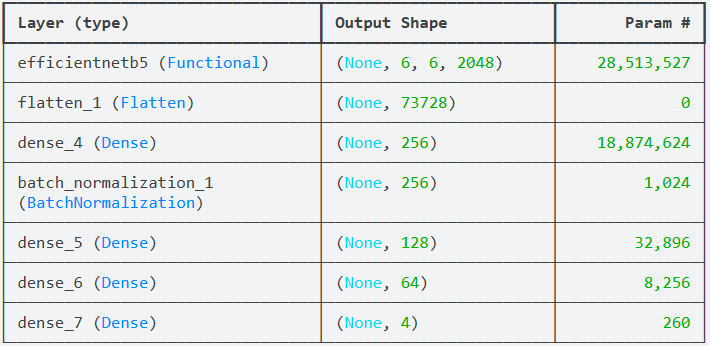AI Visual Insight: The image shows the model summary, focusing on the EfficientNetB5 backbone, flatten layer, dense layers, and output layer parameter counts. This is useful for estimating model complexity and GPU memory requirements.

Training and evaluation results show that the model generalizes well

The project trains for 30 epochs with a batch size of 32. According to the original summary, training accuracy reaches 97.79%, test accuracy is about 97.40%, and test loss is about 0.0974. These results indicate strong practical value.

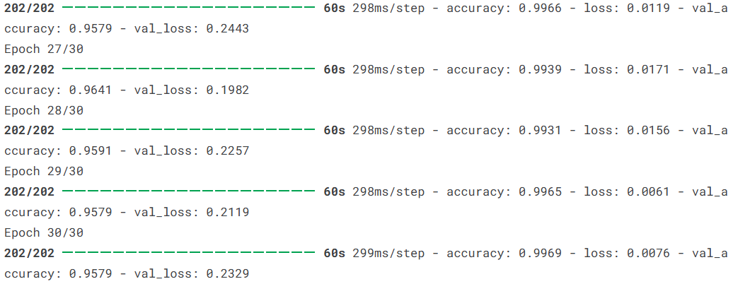AI Visual Insight: The image appears to be a screenshot of training logs that record loss and accuracy changes across epochs, which helps determine whether the model converges stably.

history = model.fit(
    X_train, y_train,
    validation_data=(X_val, y_val),
    epochs=30,
    batch_size=32,
    verbose=1
)

test_loss, test_acc = model.evaluate(X_test, y_test)
print(f'Test loss: {test_loss:.4f}, Test accuracy: {test_acc:.4f}')

This code runs model training and independent testing, which is the standard workflow for obtaining final generalization metrics.

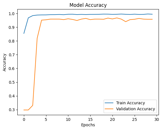AI Visual Insight: The image shows the training and validation accuracy curves. If both rise together with only a small gap, the model is learning effectively and keeping overfitting under control.

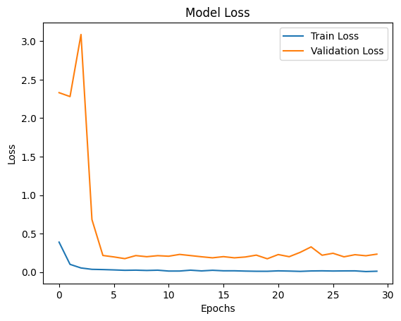AI Visual Insight: The image shows the training and validation loss curves. A steady downward trend that stabilizes over time suggests that optimization is working and the model is approaching convergence.

A confusion matrix can pinpoint class-specific error patterns

Accuracy alone is not enough. A confusion matrix answers the more important question: which class is most likely to be confused with another? This matters especially in agricultural diagnosis, where misclassifying a severe disease case as healthy carries the highest cost.

AI Visual Insight: The image appears to be a confusion matrix heatmap. Darker diagonal cells represent a higher number of correct classifications, while off-diagonal cells reveal disease-specific misclassification patterns.

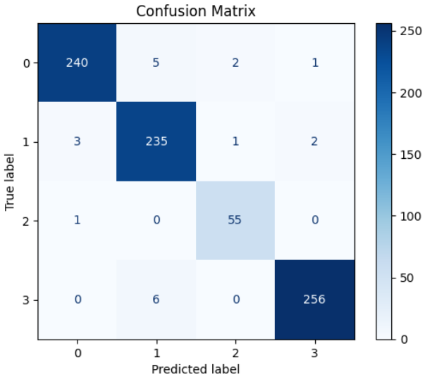AI Visual Insight: This image may show a numeric confusion matrix or a supplementary evaluation plot, further exposing classification distributions and bias sources across the four disease categories in the test set.

Random prediction visualization demonstrates intuitive interpretability

At the end of the project, nine test images are randomly sampled to compare predicted labels with ground-truth labels, with colors used to indicate correctness. This presentation works well for pre-deployment acceptance reviews.

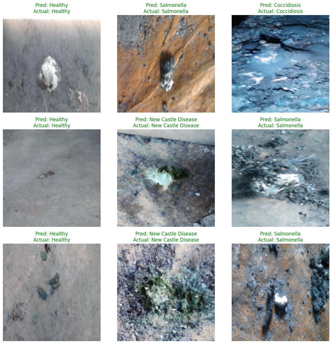AI Visual Insight: The image shows a 3×3 grid of prediction results. Each sample includes Pred and Actual labels. Green titles indicate correct predictions, while red titles indicate misclassifications, making failure patterns easy to spot.

pred = model.predict(X_test)
pred_idx = np.argmax(pred, axis=1)  # Select the class with the highest probability
true_idx = np.argmax(y_test, axis=1)

This code extracts predicted class indices and can be used for confusion matrices, error analysis, and frontend display.

Exporting the model structure helps documentation and deployment review

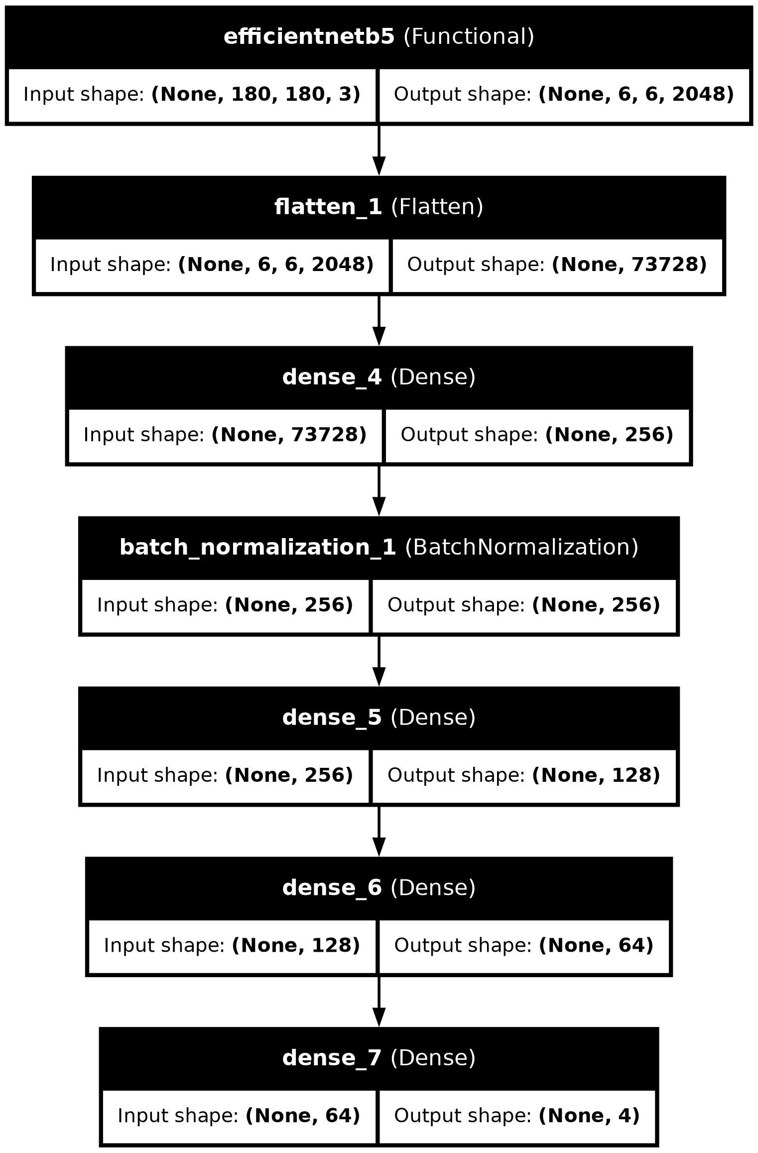AI Visual Insight: The image shows the model architecture diagram with the input layer, EfficientNetB5 backbone, and multi-layer dense classification head clearly labeled. It is suitable for reporting, reproduction, and production review.

from tensorflow.keras.utils import plot_model

plot_model(
    model,
    to_file='model_architecture.png',
    show_shapes=True,
    show_layer_names=True
)

This code saves the network structure as an image, which supports team collaboration and engineering handoff.

This project shows that transfer learning can significantly improve diagnostic efficiency in smart poultry farming

From a practical perspective, this solution delivers three core strengths: real-world data, a mature transfer learning backbone, and a highly interpretable evaluation loop. It works well both as an image classification teaching example and as an agricultural AI prototype system.

If you want to optimize it further, prioritize the following improvements: add EarlyStopping and ModelCheckpoint, address class imbalance, introduce Grad-CAM heatmaps, and package the model as a mobile or web inference service.

FAQ: The three questions developers care about most

1. Why choose EfficientNetB5 instead of ResNet or MobileNet?

EfficientNetB5 offers a better balance between parameter efficiency and accuracy, especially for fine-grained disease image classification. Compared with lighter networks, it usually captures richer texture features.

2. What parts of the original project code need the most correction?

There are three main issues: inconsistent variable names, the risk of duplicate normalization, and repeated compile calls. In addition, if you already use one-hot labels, the loss function should remain categorical_crossentropy.

3. Can this model be deployed directly on a farm?

It can serve as a prototype, but production deployment still requires more field data, evaluation under different lighting conditions and device biases, and mechanisms for inference latency control, fault tolerance, and model updates.

AI Readability Summary

This article reconstructs an EfficientNetB5-based poultry disease image classification project end to end. It covers the data source, preprocessing, transfer learning model design, training evaluation, and visual analysis for a low-cost disease warning scenario in smart poultry farming. Keywords: EfficientNetB5, transfer learning, poultry disease recognition.