This project implements multi-UAV cooperative payload transport in Matlab. Its core capabilities include 3D RRT obstacle avoidance, synchronized dual-drone handoff, and EKF-based mass estimation to address path generation, payload uncertainty, and cooperative control accuracy in complex environments. Keywords: multi-UAV collaboration, 3D RRT, dynamic control.
Technical Specification Snapshot
| Parameter | Description |
|---|---|
| Development Language | Matlab |
| Core Protocols / Mechanisms | Hierarchical control, synchronized dual-drone triggering, EKF state estimation |
| Star Count | Not provided in the source |
| Runtime Environment | Matlab + Unity 3D scene |
| Core Dependencies | RRT path planning, PID control, EKF, B-spline smoothing |
| Task Type | Multi-UAV cooperative transport and path planning |
This solution targets cooperative transport in complex 3D environments
The main challenge in multi-UAV cooperative transport is not simply getting the aircraft airborne, but enabling them to complete a transport mission together with stability and precision. The original implementation organizes the system around three core constraints: path planning, handoff synchronization, and payload estimation, forming a relatively complete research workflow.
This approach is especially suitable for logistics delivery, disaster response, and unknown-payload handling scenarios. Compared with single-UAV transport, multi-UAV collaboration increases payload capacity, but it also introduces stricter spatiotemporal synchronization requirements and more complex control coupling.
The hierarchical control architecture forms the backbone of the system
The solution divides the system into a task planning layer, a path planning layer, and a low-level control layer. The task layer defines phases such as pickup, transport, and handoff. The path layer generates feasible trajectories in 3D obstacle environments. The control layer handles trajectory tracking and parameter updates.
This layered design delivers two direct benefits. First, it reduces overall system complexity. Second, it allows planning and control modules to evolve independently. For research reproduction, this structure also makes it easier to replace individual modules, such as swapping RRT for RRT* or MPC.
% Loop through task segments and generate a path for each transport phase
for GENERAL = 1:3
    start = travel(GENERAL,1:3);   % Read the start point of the current phase
    goal  = travel(GENERAL,4:6);   % Read the goal point of the current phase

    [NODELIST, PATH, COORD_PATH, found] = RRT(start, goal, a, ...
        meshes_vector, delta, check_line, range_goal); % Run 3D RRT search

    TOTAL_COORD_PATH = [TOTAL_COORD_PATH; COORD_PATH]; % Concatenate the global path
end
This code splits the transport mission into multiple phases and runs RRT path search independently for each segment.
3D RRT generates flyable paths in obstacle-rich environments
The original implementation uses a 3D Rapidly-Exploring Random Tree algorithm for obstacle-avoidance planning. Its key parameters include the internal iteration count a=4000, expansion step size delta=5, goal threshold radius range_goal=3, and the line-segment collision sampling count check_line=5.
RRT offers simple modeling and works well in high-dimensional spaces with complex obstacle distributions. However, it naturally tends to produce angular, suboptimal paths. To address this limitation, the original solution applies trajectory smoothing after the search stage.
Seventh-order polynomial smoothing reduces path jitter
The original code does not command the UAV to fly directly through discrete nodes. Instead, it first constructs a seventh-order polynomial interpolation and then generates a continuous trajectory. This makes it possible to constrain position, velocity, acceleration, and jerk boundary conditions at the same time, reducing abrupt demands on the controller.
numpts_for_segment = 1000;
lin = linspace(0,1,numpts_for_segment); % Generate a normalized time axis

A = [1 0 0 0 0 0 0 0;
     1 1 1 1 1 1 1 1;
     0 1 0 0 0 0 0 0;
     0 1 2 3 4 5 6 7;
     0 0 2 0 0 0 0 0;
     0 0 2 6 12 20 30 42;
     0 0 0 6 0 0 0 0;
     0 0 0 9 24 60 120 210];

b = [0 1 0 0 0 0 0 0]';            % Boundary state constraints
ai = A \ b;                         % Solve the seventh-order polynomial coefficients
s_t = ai(8)*lin.^7 + ai(7)*lin.^6 + ai(6)*lin.^5 + ai(5)*lin.^4 + ...
      ai(4)*lin.^3 + ai(3)*lin.^2 + ai(2)*lin + ai(1);
This code generates a trajectory interpolation curve with high-order continuity, making it suitable for smooth UAV tracking.
The dual-drone synchronization mechanism determines whether handoff remains stable and reliable
Cooperative transport is not just about having two paths that exist at the same time. The two UAVs must complete payload transfer with precise timing consistency near the handoff point. The original solution uses a distance-threshold trigger: when the distance between the two UAVs falls below dsync, the first UAV releases the payload and the second UAV takes over.
This type of design is simple to implement and common in engineering practice. However, it depends heavily on localization accuracy and control latency. If attitude error is significant, or if communication jitter is present, payload swing or even drop risk may occur at the handoff point. In practice, synchronization compensation usually requires PID or more advanced relative pose control.
Online EKF mass estimation improves control robustness under unknown payloads
One of the hardest parts of a transport mission is that the payload mass may be unknown. If the controller continues allocating thrust using a fixed mass parameter, the system can experience altitude error, attitude overshoot, or even instability. The original implementation uses an Extended Kalman Filter to estimate mass online and feeds the estimated value back into the controller in real time.
 AI Visual Insight: This figure shows the core form of the EKF state update equation, highlighting how the system prior estimate is fused with sensor observations through the Kalman gain. In this project, that means the UAV can continuously refine payload mass estimation based on thrust, acceleration, and sensor feedback, then dynamically update control parameters.
The estimated mass directly affects thrust and attitude allocation
The control layer updates the thrust equation F = m · (g + a) using the estimated mass. When the payload becomes heavier, the system automatically increases thrust demand. As the estimate gradually converges, attitude control also becomes more stable. According to the original experiment, when the true mass is 5 kg and the initial estimate is 3 kg, the EKF converges in about 10 seconds with a steady-state error below 0.2 kg.
m_est = 3.0;                 % Initial mass estimate
g = 9.81;
a_cmd = [0; 0; 1.2];         % Desired acceleration

F_cmd = m_est * (g + a_cmd(3)); % Update total thrust using the estimated mass
This code shows how mass estimation directly enters the control allocation loop.
The experimental results demonstrate baseline feasibility
The original experiment uses a Unity 3D obstacle environment, a payload with a true mass of 5 kg, and a synchronization threshold of 1 m. The reported results show that the average RRT planning time is about 2.3 seconds, dual-drone handoff error remains below 0.5 m, and synchronization time stays under 3 seconds.
 AI Visual Insight: This figure appears to show UAV trajectories or stage-based path results in a 3D environment. It is typically useful for examining start and goal distribution, obstacle bypass trends, and the spatial continuity of trajectory segments to validate RRT reachability in complex spaces.
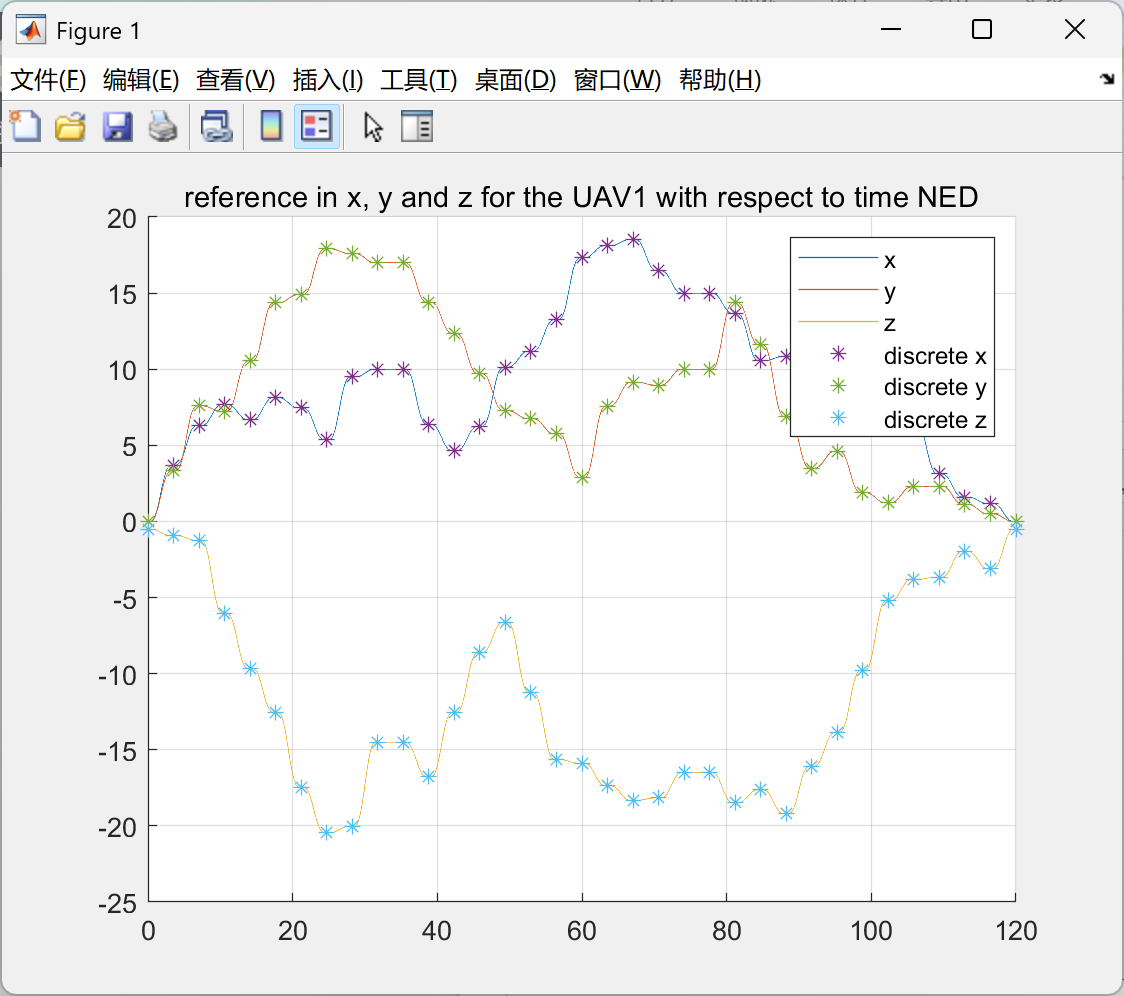
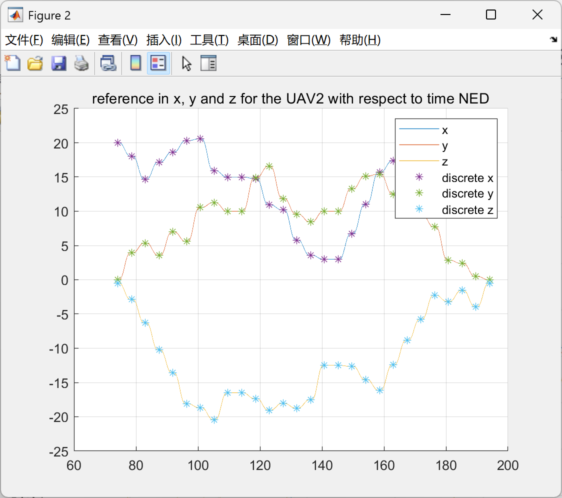 AI Visual Insight: This figure most likely reflects control response or trajectory tracking behavior and can be used to assess whether the smoothed interpolation introduces noticeable oscillation, overshoot, or abrupt transitions between phases.
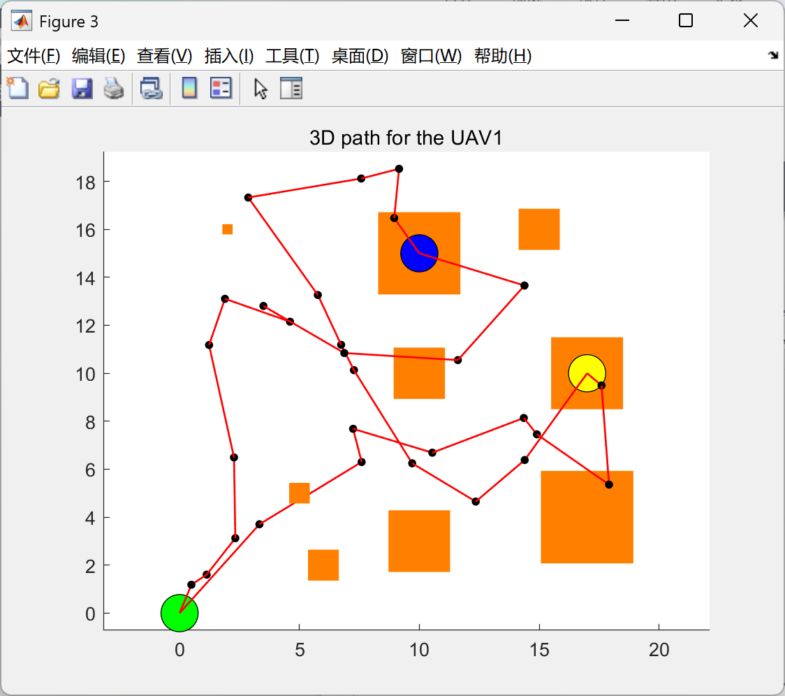 AI Visual Insight: This figure may show the overall route layout after concatenating multi-stage task paths, helping analyze whether pickup, transport, and handoff phases connect continuously and whether local detours are present.
These metrics indicate that the system already covers three essential capabilities: planning, handoff, and payload estimation. However, it remains a research-validation implementation and still falls short of production deployment in terms of stability and real-time performance.
This implementation still has three clear optimization paths
First, path planning can be upgraded to RRT*, PRM, or MPC-based online replanning to improve path quality and real-time responsiveness. Second, dual-drone coordination can incorporate relative navigation and predictive control to reduce handoff error. Third, the visualization layer can use higher-fidelity 3D animation to strengthen experimental interpretability.
For paper reproduction, the value of this Matlab solution lies in its clear structure and well-defined module boundaries. For production engineering, it still needs stronger sensor noise modeling, communication delay compensation, and collision-safety redundancy.
FAQ
1. Why use RRT here instead of A*?
RRT is better suited to continuous 3D spaces and complex obstacle environments, and it does not depend on a regular grid. A* is more intuitive on discrete maps, but its expansion cost becomes higher in high-dimensional continuous spaces.
2. Why is online mass estimation necessary?
Because when payload mass is unknown, a fixed-thrust model introduces control bias. EKF continuously corrects the mass parameter based on observations, allowing thrust and attitude control to better match the real system.
3. Can this solution scale to three or more UAVs?
Yes, but the challenge shifts from dual-drone synchronization to multi-UAV spatiotemporal consistency and collision-avoidance coordination. This requires additional mechanisms for task allocation, relative formation constraints, and communication consistency.
Core Summary: This article reconstructs a Matlab-based multi-UAV cooperative transport solution centered on three modules: 3D RRT obstacle avoidance, synchronized dual-drone handoff, and EKF mass estimation. It explains the hierarchical control architecture, key parameters, experimental performance, and optimization directions, making it a practical starting point for research in UAV cooperative control and path planning.