AI Readability Summary: This article reconstructs the core knowledge chain of multivariable differential calculus, covering double limits, partial derivatives, total differentials, implicit differentiation, gradients, and extrema tests. It addresses scattered formulas, broken logical flow, and the difficulty of transferring solution methods across examples. Keywords: multivariable functions, partial derivatives, Lagrange multipliers.
Technical Specification Snapshot
| Parameter | Content |
|---|---|
| Subject / Language | Advanced Mathematics / Chinese |
| Core Topic | Multivariable Differential Calculus and Its Applications |
| Format Protocol | Markdown + LaTeX-style formulas |
| Original Source Characteristics | Organized CSDN math notes |
| Star Count | N/A |
| Core Dependencies | Limit theory, derivative definitions, basic linear algebra |
Multivariable differential calculus forms the backbone of 2D and 3D analysis
The objects of study in multivariable functions extend from single-variable cases to two, three, or even higher dimensions. The key shift is not simply that “there are more variables,” but that limit paths, local linearization, and geometric interpretation all become more complex at the same time.
In engineering computation, computer vision, optimization modeling, and physical field analysis, partial derivatives, gradients, and extrema tests are among the most frequently used tools. For that reason, building a knowledge chain from definitions to applications matters far more than memorizing isolated formulas.
A quick knowledge framework to remember
Point sets and neighborhoods → Double limits → Continuity → Partial derivatives → Total differential
→ Composite differentiation → Implicit differentiation → Directional derivatives and gradients → Extrema and constrained optimization
This chain describes the shortest learning path through multivariable calculus.
Point sets, neighborhoods, and domains determine the boundaries of discussion
On the plane, a point set can be written as (E={(x,y)\mid P(x,y)}). A neighborhood around the point ((x_0,y_0)) consists of all points whose distance from that point is less than (\delta). A punctured neighborhood excludes the center point itself.
From this, we can define interior points, exterior points, boundary points, and accumulation points. These then lead to concepts such as open sets, closed sets, connected sets, regions, and bounded sets. These terms determine whether a limit can be discussed and whether the maximum-minimum theorem applies.
Understanding neighborhood tests with code
def in_neighborhood(x, y, x0, y0, delta):
    # Check whether a point lies inside the neighborhood centered at (x0, y0)
    return ((x - x0)**2 + (y - y0)**2) ** 0.5 < delta

def in_punctured_neighborhood(x, y, x0, y0, delta):
    # A punctured neighborhood requires distance greater than 0 and less than delta
    d = ((x - x0)**2 + (y - y0)**2) ** 0.5
    return 0 < d < delta
This code corresponds directly to the formal definitions of a neighborhood and a punctured neighborhood.
The essence of a double limit is that path independence must hold
Suppose (f(x,y)) is defined near the point ((x_0,y_0)). If, whenever ((x,y)) approaches that point in any manner, the function value approaches the same constant (A), then the limit is said to exist.
The most important test idea is not “find one path along which the limit works,” but rather “rule out all path-dependent differences.” As long as two paths produce different results, the limit does not exist.
A classic counterexample makes path dependence obvious
def f(x, y):
    # Define the origin separately as 0; use the rational expression elsewhere
    if x == 0 and y == 0:
        return 0
    return x * y / (x * x + y * y)

# Along y = x, the function value is always 1/2
# Along y = -x, the function value is always -1/2
This function approaches different values along different paths toward the origin, so the double limit does not exist.
Continuity requires the limit value to match the function value exactly
If (\lim_{(x,y)\to(x_0,y_0)}f(x,y)=f(x_0,y_0)), then the function is continuous at that point. Continuity is an important prerequisite for partial derivatives, differentiability, geometric approximation, and extrema theory.
On a bounded closed region, a continuous function must be bounded, must attain both a maximum and a minimum, and satisfies the intermediate value property and uniform continuity. This provides the theoretical foundation for later extrema problems.
Partial derivatives characterize local rates of change under single-variable perturbations
A partial derivative is, in essence, a derivative taken while holding the other variables fixed and allowing only one variable to change. (f_x) describes the instantaneous rate of change in the x-direction, and (f_y) describes the instantaneous rate of change in the y-direction.
But one point requires special attention: the existence of all partial derivatives at a point does not necessarily imply continuity, and it certainly does not necessarily imply differentiability. This is one of the most easily confused differences between multivariable calculus and single-variable calculus.
A symbolic example of partial derivative computation
import sympy as sp

x, y = sp.symbols('x y')
z = x**2 * y + sp.sin(x * y)

zx = sp.diff(z, x)  # Compute the partial derivative with respect to x
zy = sp.diff(z, y)  # Compute the partial derivative with respect to y
print(zx, zy)
This code demonstrates the mechanical computation of partial derivatives.
The total differential gives a local linear approximation of a multivariable function
If a function is differentiable at ((x,y)), then its increment can be written as (\Delta z = f_x(x,y)\Delta x + f_y(x,y)\Delta y + o(\rho)). The first two terms form the principal linear part, while the remainder is of higher order relative to (\rho).
Therefore, the total differential is: (dz=f_xdx+f_ydy). This is not just a formula to memorize. It is the best local linear approximation. Continuity of the partial derivatives is a commonly used sufficient condition for differentiability.
Composite differentiation must propagate step by step along the dependency chain
If (z=f(u,v)), and (u=\phi(x,y), v=\psi(x,y)), then (\frac{\partial z}{\partial x}=\frac{\partial z}{\partial u}\frac{\partial u}{\partial x}+\frac{\partial z}{\partial v}\frac{\partial v}{\partial x}). The partial derivative with respect to y follows in the same way.
This is the chain rule expanded into the multivariable setting. In essence, it is gradient propagation over a dependency graph, which closely mirrors the backpropagation idea used in modern automatic differentiation frameworks.
A concise implementation of composite differentiation
import sympy as sp

x, y = sp.symbols('x y')
u = x * y
v = x + y
z = sp.exp(u) * sp.sin(v)

zx = sp.diff(z, x)  # Automatically expands the chain rule
zy = sp.diff(z, y)  # Computes the partial derivative with respect to y
print(sp.simplify(zx), sp.simplify(zy))
This code is equivalent to applying the multivariable chain rule by hand.
Implicit differentiation turns non-explicit relations into computable derivatives
When the equation (F(x,y)=0) satisfies (F_y\neq 0) at a point, it locally determines a unique implicit function (y=f(x)), and (\frac{dy}{dx}=-\frac{F_x}{F_y}).
In the three-variable case, if (F(x,y,z)=0) and (F_z\neq 0), then (\frac{\partial z}{\partial x}=-\frac{F_x}{F_z}), (\frac{\partial z}{\partial y}=-\frac{F_y}{F_z}).
This method avoids solving explicitly before differentiating, which makes it especially useful in geometric problems involving circles, spheres, surfaces, and intersection curves.
Directional derivatives and gradients reveal the direction of fastest change
A directional derivative describes the rate of change of a function along a unit direction (l): (\frac{\partial f}{\partial l}=f_x\cos\alpha+f_y\cos\beta).
The gradient is defined as (\nabla f=(f_x,f_y)). It points in the direction of steepest increase, and its magnitude equals the maximum directional derivative. This result is critically important in optimization, image edge detection, and physical field analysis.
A minimal example of gradient computation
import sympy as sp

x, y = sp.symbols('x y')
f = x**2 + y**2 - 1

grad = [sp.diff(f, x), sp.diff(f, y)]  # Gradient vector
print(grad)
This code outputs the gradient expression of the function at any point.
Extrema tests depend on critical points and the Hessian-type second-derivative criterion
If a function is differentiable at an extremum point, then it must satisfy (f_x=f_y=0). This is only a necessary condition and is not enough to draw a conclusion on its own.
Let (A=f{xx}, B=f{xy}, C=f_{yy}), and form the discriminant (AC-B^2). If it is greater than 0, an extremum exists; in that case, (A>0) indicates a local minimum and (A<0) indicates a local maximum. If it is less than 0, the point is not an extremum.
Under a constraint (\phi(x,y)=0), we should construct the Lagrangian (L(x,y,\lambda)=f(x,y)+\lambda\phi(x,y)), and then solve the first-order conditions together to find candidate points.
Multivariable differential calculus ultimately unifies around geometry and optimization
From tangent lines and normal planes to space curves, to tangent planes and normal lines to surfaces, and then to directional derivatives, gradient fields, and constrained extrema, all formulas revolve around one central idea: the local rate of change.
For that reason, the most effective way to learn this topic is not rote memorization, but reducing every concept to three questions: along which direction does change occur, how is the rate of change defined, and can it be approximated by a linear model?
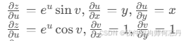 AI Visual Insight: The image shows a handwritten derivation of the total differential expansion for a composite function. The core idea is to first write the differentials of the intermediate variables (u,v) with respect to (x,y), then substitute them back into (dz=\frac{\partial z}{\partial u}du+\frac{\partial z}{\partial v}dv), and finally collect the linear terms in (dx,dy). This gives an intuitive explanation of how the “invariance of the total differential form” becomes the familiar partial-derivative expression.
 AI Visual Insight: The animated image works more as a conceptual aid for understanding extrema of multivariable functions or constrained optimization. It emphasizes the geometric relationship between variable changes and the objective surface. Although the resolution is limited, its technical meaning typically corresponds to tangent level curves, collinear gradients, or a dynamic illustration of extremum locations in the Lagrange multiplier method.
FAQ
1. Why does the existence of a limit along one path not imply that the full multivariable limit exists?
Because a double limit requires convergence to the same value along every possible path. One path can only provide local evidence; it cannot cover all possible approaches.
2. Why does the existence of partial derivatives not guarantee differentiability?
Because partial derivatives only show that rates of change exist along coordinate-axis directions, while differentiability requires the function to be approximated by a single linear map in all sufficiently small directions. That condition is stronger.
3. What are the most common practical uses of the gradient?
The gradient is commonly used in steepest-ascent search, loss function optimization, image edge detection, potential field analysis, and surface normal computation.
Core Summary: This article systematically organizes the core framework of multivariable differential calculus in advanced mathematics, covering point sets and domains, double limits, continuity, partial derivatives, total differentials, composite differentiation, implicit differentiation, directional derivatives, gradients, and the Lagrange multiplier method, together with representative examples and formula memorization shortcuts.